目录
一 安装
1.1 装包
SCENIC的workflow主要依赖三个R包的支持:
1、GENIE3:用于共表达网络的计算(也可以用GRNBoost2替代)
2、RcisTarget:转录因子结合motif的计算
3、AUCell:识别单细胞测序数据中的激活基因集(gene-network)
#安装是个永恒的难题,我在window中BiocManager==1.30.16,R==4.0.6以及本篇的sessionInfo环境下安装是没有问题的
#在Linux中如果你对conda比较熟悉那么也很好安装
if (!requireNamespace("BiocManager", quietly = TRUE))install.packages("BiocManager")
BiocManager::version()
#当你的bioconductor版本大于4.0时
if(!require(SCENIC))BiocManager::install(c("AUCell", "RcisTarget"),ask = F,update = F);BiocManager::install(c("GENIE3"),ask = F,update = F)#这三个包显然是必须安装的

### 可选的包:
#AUCell依赖包
if(!require(SCENIC))BiocManager::install(c("zoo", "mixtools", "rbokeh"),ask = F,update = F)
###t-SNEs计算依赖包:
if(!require(SCENIC))BiocManager::install(c("DT", "NMF", "ComplexHeatmap", "R2HTML", "Rtsne"),ask = F,update = F)

# #这几个包用于并行计算,很遗憾,Windows下并不支持,所以做大量数据计算时最好转战linux:
if(!require(SCENIC))BiocManager::install(c("doMC", "doRNG"),ask = F,update = F)
#可视化输出

# To export/visualize in http://scope.aertslab.org
if (!requireNamespace("devtools", quietly = TRUE))install.packages("devtools")
if(!require(SCopeLoomR))devtools::install_github("aertslab/SCopeLoomR", build_vignettes = TRUE)#SCopeLoomR用于获取测试数据

if (!requireNamespace("arrow", quietly = TRUE)) BiocManager::install('arrow')
#这个包不装上在runSCENIC_2_createRegulons那一步会报错,提示'dbs'不存在
library(SCENIC)#这就安装好了,试试能不能正常加载

if(!require(SCENIC))devtools::install_github("aertslab/SCENIC")
packageVersion("SCENIC")#这里我安装的是1.3.1
library(SCENIC)

#bioconductor版本小于4.0或你的R(3.6)的版本也比较老,你可能得试试下面的方法进行安装
devtools::install_github("aertslab/[email protected]")
devtools::install_github("aertslab/AUCell")
devtools::install_github("aertslab/RcisTarget")
devtools::install_github("aertslab/GENIE3")
1.2 官方手册
vignetteFile <- file.path(system.file('doc', package='SCENIC'), "SCENIC_Running.Rmd")
file.copy(vignetteFile, "SCENIC_myRun.Rmd")
# or:
vignetteFile <- "https://raw.githubusercontent.com/aertslab/SCENIC/master/vignettes/SCENIC_Running.Rmd"
download.file(vignetteFile, "SCENIC_myRun.Rmd")
1.3 测试数据
1.3.1 从测试数据中提取表达矩阵与注释信息
输入数据的表达矩阵为gene-summarized counts,不同于其他进阶分析的是,输入的数据最好是raw counts或normalized counts。计算后的TPM或FPKM/RPKM之类也是允许的, 但是这些可能会导致人为的共变量引入,避免节外生枝,我还是推荐用raw count。但总的来说, raw (logged) UMI counts, normalized UMI counts, 和TPM都能产生值得信赖的效果 form loom
loomPath <- system.file(package="SCENIC", "examples/mouseBrain_toy.loom")
library(SCopeLoomR)
loom <- open_loom(loomPath)#获取loom文件
exprMat <- get_dgem(loom)#取出表达信息
class(exprMat)# [1] "matrix" "array"exprMat[1:4,1:4]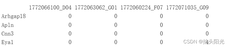
cellInfo <- get_cell_annotation(loom)#获得注释信息
cellInfo[1:4,1:3] 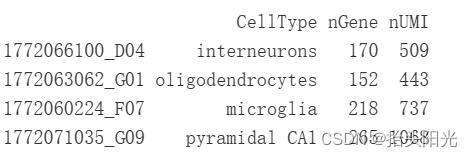
close_loom(loom)上面我们说了如何从loom中读取表达矩阵与注释信息,而Python版的SCENIC是推荐使用loom作为输入数据的,这里教大家如何利用表达矩阵和注释信息创建loom文件(to loom)
loom <- build_loom("data/mouseBrain.loom", dgem=exprMat)
loom <- SCENIC::add_cell_annotation(loom, cellInfo)close_loom(loom) seurat对象也是类似的
library(Seurat)
singleCellMatrix <- Seurat::Read10X(data.dir="data/filtered_gene_bc_matrices/hg19/")
scRNAsub <- CreateSeuratObject(counts = singleCellMatrix, project = "pbmc3k", min.cells = 3, min.features = 200)
exprMat <- as.matrix(scRNAsub@assays$RNA@counts)
cellInfo <- as.data.frame([email protected])从AUCell中读取注释信息
cellLabels <- paste(file.path(system.file('examples', package='AUCell')), "mouseBrain_cellLabels.tsv", sep="/")
cellLabels <- read.table(cellLabels, row.names=1, header=TRUE, sep="\t")
cellInfo <- as.data.frame(cellLabels)
colnames(cellInfo) <- "CellType"
saveRDS(cellInfo,'int/cellInfo.rds')
1.3.2 保存输入数据
saveRDS(cellInfo, file="int/cellInfo.Rds")
# Color to assign to the variables (same format as for NMF::aheatmap)
colVars <- list(CellType=c("microglia"="forestgreen",
                           "endothelial-mural"="darkorange",
                           "astrocytes_ependymal"="magenta4",
                           "oligodendrocytes"="hotpink",
                           "interneurons"="red3",
                           "pyramidal CA1"="skyblue",
                           "pyramidal SS"="darkblue"))
colVars$CellType <- colVars$CellType[intersect(names(colVars$CellType), cellInfo$CellType)]
saveRDS(colVars, file="int/colVars.Rds")
plot.new(); legend(0,1, fill=colVars$CellType, legend=names(colVars$CellType))#查看保存了哪些细胞类型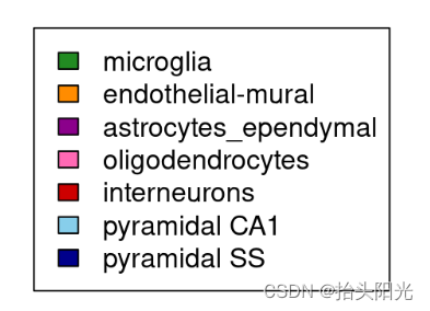
1.4 RcisTarget数据库
1.4.1 文件获取
cisTarget databases 手动下载
#地址
#human:
dbFiles <- c("https://resources.aertslab.org/cistarget/databases/homo_sapiens/hg19/refseq_r45/mc9nr/gene_based/hg19-500bp-upstream-7species.mc9nr.feather",
             "https://resources.aertslab.org/cistarget/databases/homo_sapiens/hg19/refseq_r45/mc9nr/gene_based/hg19-tss-centered-10kb-7species.mc9nr.feather")

#mouse:
dbFiles <- c("https://resources.aertslab.org/cistarget/databases/mus_musculus/mm9/refseq_r45/mc9nr/gene_based/mm9-500bp-upstream-7species.mc9nr.feather",
             "https://resources.aertslab.org/cistarget/databases/mus_musculus/mm9/refseq_r45/mc9nr/gene_based/mm9-tss-centered-10kb-7species.mc9nr.feather")


#fly:
dbFiles <- c("https://resources.aertslab.org/cistarget/databases/drosophila_melanogaster/dm6/flybase_r6.02/mc8nr/gene_based/dm6-5kb-upstream-full-tx-11species.mc8nr.feather")

#下载

dir.create("cisTarget_databases"); setwd("cisTarget_databases")
for(featherURL in dbFiles)
{
  download.file(featherURL, destfile=basename(featherURL)) # saved in current dir
}
1.4.2 RcisTarget数据库文件初始化
这一步相当于给上面下好的文件构建索引并设置一些默认参数
### Initialize settings
library(SCENIC)
scenicOptions <- initializeScenic(org="mgi",#mouse填'mgi', human填'hgnc',fly填'dmel')
dbDir="cisTarget_databases/mouse/mouse.mm9/", nCores=8)#这里可以设置并行计算
scenicOptions@inputDatasetInfo$cellInfo <- "int/cellInfo.Rds"
saveRDS(scenicOptions, file="int/scenicOptions.Rds")
二、 SCENIC分析流程(精简版)
SCENIC的分析流程封装的较好,运行完整个流程无非也十几行代码(但是会产生大量的过程及结果文件)。
下面这个示例数据真的算的很快,不过大家跑自己数据时可能会算上好几天。
loomPath <- system.file(package="SCENIC", "examples/mouseBrain_toy.loom")
library(SCopeLoomR)
loom <- open_loom(loomPath)#获取loom文件
exprMat <- get_dgem(loom)#取出表达信息
cellInfo <- get_cell_annotation(loom)#获得注释信息2.1. 计算共表达网络
genesKept <- geneFiltering(exprMat, scenicOptions)
exprMat_filtered <- exprMat[genesKept, ]
runCorrelation(exprMat_filtered, scenicOptions)
exprMat_filtered_log <- log2(exprMat_filtered+1)
# 基因共表达网络计算
mymethod <- 'runGenie3' # 'grnboost2'
library(reticulate)
if(mymethod=='runGenie3'){
runGenie3(exprMat_filtered_log, scenicOptions)
}else{
arb.algo = import('arboreto.algo')
tf_names = getDbTfs(scenicOptions)
tf_names = Seurat::CaseMatch(
search = tf_names,
match = rownames(exprMat_filtered))
adj = arb.algo$grnboost2(
as.data.frame(t(as.matrix(exprMat_filtered))),
tf_names=tf_names, seed=2023L
)
colnames(adj) = c('TF','Target','weight')
saveRDS(adj,file=getIntName(scenicOptions,
'genie3ll'))
}
2.2. 构建并计算基因调控网络活性(GRN score)
exprMat_log <- log2(exprMat+1)
scenicOptions@settings$dbs <- scenicOptions@settings$dbs["10kb"] # Toy run settings
scenicOptions <- runSCENIC_1_coexNetwork2modules(scenicOptions)
scenicOptions <- runSCENIC_2_createRegulons(scenicOptions, coexMethod=c("top5perTarget")) # Toy run settings
scenicOptions <- runSCENIC_3_scoreCells(scenicOptions, exprMat_log)
# 通过交互的shiny app选择判定二元矩阵的阈值,这里Rmarkdown不便展示,大家可以自行尝试一下
# aucellApp <- plotTsne_AUCellApp(scenicOptions, exprMat_log)
# savedSelections <- shiny::runApp(aucellApp)
# newThresholds <- savedSelections$thresholds
# scenicOptions@fileNames$int["aucell_thresholds",1] <- "int/newThresholds.Rds"
# saveRDS(newThresholds, file=getIntName(scenicOptions, "aucell_thresholds"))

scenicOptions <- runSCENIC_4_aucell_binarize(scenicOptions)#将AUCell矩阵二元化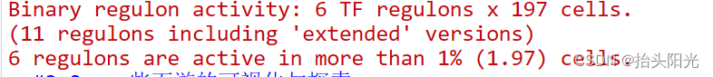
2.3. 一些下游的可视化与探索
tsneAUC(scenicOptions, aucType="AUC") #利用AUCell score运行tsne![]()
# Export:
# saveRDS(cellInfo, file=getDatasetInfo(scenicOptions, "cellInfo")) # Temporary, to add to loom
if(!file.exists('output/scenic.loom')){export2loom(scenicOptions, exprMat)}

saveRDS(scenicOptions, file="int/scenicOptions.Rds")#保存结果

### Exploring output
# output下存放的scenic.loom文件可以用这个网站做交互式的可视化: http://scope.aertslab.org

# motif富集的相关信息在:
#output/Step2_MotifEnrichment_preview.html in
motifEnrichment_selfMotifs_wGenes <- loadInt(scenicOptions, "motifEnrichment_selfMotifs_wGenes")
tableSubset <- motifEnrichment_selfMotifs_wGenes[highlightedTFs=="Sox8"]#这样查看Sox8的信息
viewMotifs(tableSubset) 
#查看motif和对应基因:
#output/Step2_regulonTargetsInfo.tsv
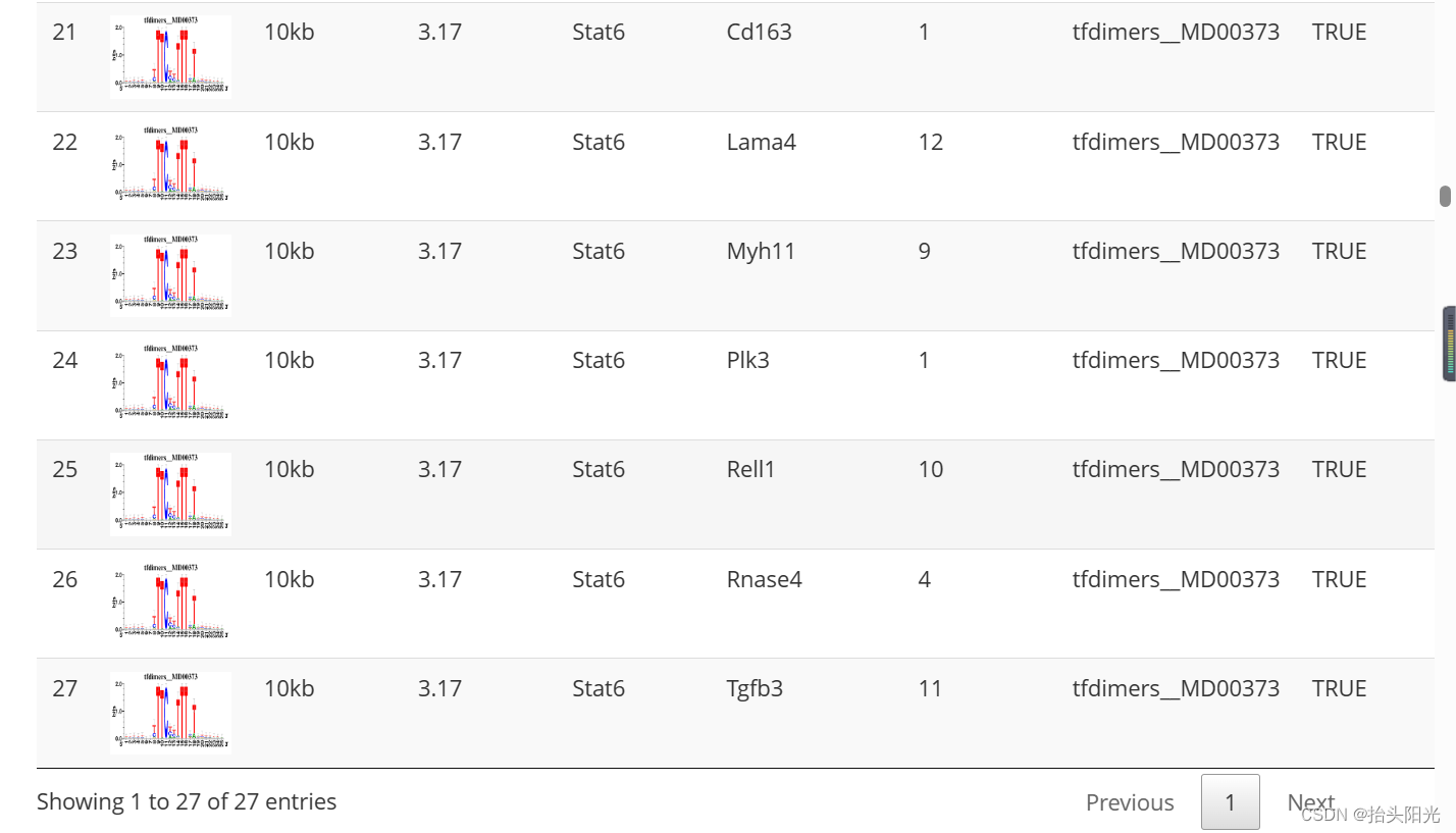
regulonTargetsInfo <- loadInt(scenicOptions, "regulonTargetsInfo")
tableSubset <- regulonTargetsInfo[TF=="Stat6" & highConfAnnot==TRUE]
viewMotifs(tableSubset) 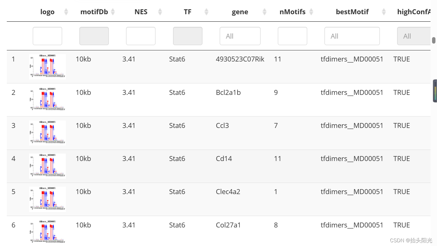
#计算并展示每种细胞类型特异性的(celltype Cell-type specific regulators (RSS)),类似于拿RGN的活性来计算调控
regulonAUC <- loadInt(scenicOptions, "aucell_regulonAUC")
rss <- calcRSS(AUC=getAUC(regulonAUC), cellAnnotation=cellInfo[colnames(regulonAUC), "CellType"], )
rssPlot <- plotRSS(rss)
plotly::ggplotly(rssPlot$plot)
2.4 输出文件
除了我们上面可视化展示出的结果,SCENIC运行时会自动在本地输出大量文件: