利用神经风格迁移创造艺术
开发环境
作者:嘟粥yyds
时间:2023年7月17日
集成开发工具:Google Colab
集成开发环境:Python 3.10.6
第三方库:tensorflow、os、Ipython、matplotlib、PIL、time、functools、imageio
概要
本文使用深度学习来用其他图像的风格创造一个图像(曾经你是否希望可以像毕加索或梵高一样绘画?)。 这被称为神经风格迁移,该技术概述于 A Neural Algorithm of Artistic Style (Gatys et al.).
神经风格迁移是一种优化技术,主要用于获取两个图像(内容图像和风格参考图像(例如著名画家的艺术作品))并将它们混合在一起,以便使输出图像看起来像内容图像,但却是以风格参考图像的风格“绘制”的。
这是通过优化输出图像以匹配内容图像的内容统计和风格参考图像的风格统计来实现的。这些统计信息是使用卷积网络从图像中提取的。
注:本文使用的是原始的风格迁移算法。它将图像内容优化为特定风格。现代方式会训练模型以直接生成风格化图像(类似于 CycleGAN)。这种方式要快得多(最多可达 1000 倍)。
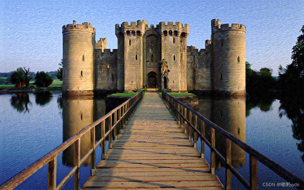
例如,让我们以下面这个城堡图像作为内容图像并以梵高的星空作为风格参考图像生成一幅风格化图像。


本文要点
- 介绍风格迁移的基本概念 - 将一张图片的内容与另一张图片的风格进行合成,创造出风格迁移后的新图像。
- 阐述风格迁移的核心思想 - 使用卷积神经网络提取内容和风格特征,将两个特征重新结合得到迁移结果。
- 概述风格迁移的算法流程 - 输入内容图片和风格图片,基于卷积神经网络提取特征,定义内容损失和风格损失,通过反向传播优化生成目标图片。
- 使用TensorFlow框架实现了风格迁移的模型 - 构建卷积神经网络,定义关键层提取内容和风格特征向量,计算损失函数,训练生成目标图像。
- 展示不同风格迁移的示例结果 - 包括照片到梵高、毕加索等艺术家风格的迁移。
- 分析风格迁移算法的优缺点 - 创造性强但计算资源消耗大,结果可控性较差等。
实现步骤
1 配置
1.1 导入和配置模块
import os
import tensorflow as tf
# 从tensorflow_hub中加载压缩格式的模型以提高加载和存储效率
os.environ['TFHUB_MODEL_LOAD_FORMAT'] = 'COMPRESSED'

import IPython.display as display  # 在Jupyter Notebook等环境中显示图像、音频、视频等内容
from IPython.display import Image

import matplotlib.pyplot as plt
import matplotlib as mpl
mpl.rcParams['figure.figsize'] = (12, 12)
mpl.rcParams['axes.grid'] = False

import numpy as np
import PIL.Image
import time
import functools
import imageio
def tensor_to_image(tensor):
  """
  将张量转换为图像。
  参数:
  - tensor: 输入的张量
  返回:
  - 转换后的 PIL 图像对象
  """
  tensor = tensor * 255 # 将张量值缩放到 0 到 255 的范围,即图像的正常表示范围
  tensor = np.array(tensor, dtype=np.uint8) # 将张量转换为 NumPy 数组,数据类型为uint8

  if np.ndim(tensor) > 3: # 检查张量的维度数,因为当维度大于3时第一维表示的是图片数
      assert tensor.shape[0] == 1 # 确保张量的第一个维度是 1
      tensor = tensor[0] # 将张量转换为单张图像

  return PIL.Image.fromarray(tensor) # 将 NumPy 数组转换为 PIL 图像对象,并返回
1.2 将输入进行可视化
def load_img(path_to_img):
  """
  加载图像文件并进行预处理。

  参数:
  - path_to_img: 图像文件的路径

  返回:
  - 预处理后的图像张量
  """
  # 定义最大的图像尺寸为 1024x1024 像素,大概需要15G的显存,若显存不足则可适当调小(例512x512需要8G左右的显存)
  max_dim = 1024
  # 读取图像文件的内容
  img = tf.io.read_file(path_to_img)
  img = tf.image.decode_image(img, channels=3) # 将图像解码为张量,并指定通道数为 3(RGB图像)
  img = tf.image.convert_image_dtype(img, tf.float32) # 将图像数据类型转换为浮点型,并将像素值归一化到 [0, 1] 范围

  shape = tf.cast(tf.shape(img)[:-1], tf.float32) # 获取图像的形状,并将其转换为浮点型
  long_dim = max(shape) # 获取图像的最长边
  scale = max_dim / long_dim # 计算缩放比例

  new_shape = tf.cast(shape * scale, tf.int32) # 计算新的图像形状

  img = tf.image.resize(img, new_shape) # 将图像按照新的形状进行缩放
  img = img[tf.newaxis, :] # 在图像张量的第一个维度上增加一个维度

  return img
def imshow(image, title=None):
  if len(image.shape) > 3:
    image = tf.squeeze(image, axis=0)

  plt.imshow(image)
  if title:
    plt.title(title)
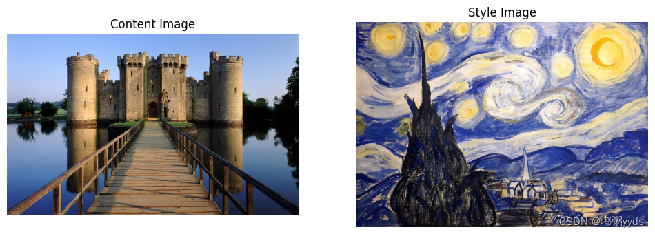
content_image = load_img('data_Neural style transfer/content.jpg')
style_image = load_img('data_Neural style transfer/style.jpg')

plt.subplot(1, 2, 1)
# 关闭坐标轴显示
plt.axis('off')
imshow(content_image, 'Content Image')

plt.subplot(1, 2, 2)
# 关闭坐标轴显示
plt.axis('off')
imshow(style_image, 'Style Image')
2 定义内容和风格的表示
使用模型的中间层来获取图像的内容和风格表示。 从网络的输入层开始,前几个层的激励响应表示边缘和纹理等低级 feature (特征)。 随着层数加深,最后几层代表更高级的 feature (特征)——实体的部分,如轮子或眼睛。 本文使用的是 VGG19 网络结构,这是一个已经预训练好的图像分类网络。 这些中间层是从图像中定义内容和风格的表示所必需的。 对于一个输入图像,我们尝试匹配这些中间层的相应风格和内容目标的表示。
加载 VGG19 并在我们的图像上测试它以确保正常运行:
x = tf.keras.applications.vgg19.preprocess_input(content_image*255)
x = tf.image.resize(x, (224, 224))
vgg = tf.keras.applications.VGG19(include_top=True, weights='imagenet')
prediction_probabilities = vgg(x)
prediction_probabilities.shape  # TensorShape([1, 1000])
predicted_top_5 = tf.keras.applications.vgg19.decode_predictions(prediction_probabilities.numpy())[0]
[(class_name, prob) for (number, class_name, prob) in predicted_top_5]
[('castle', 0.98721236),
 ('palace', 0.0058733267),
 ('suspension_bridge', 0.0025044687),
 ('church', 0.0007503911),
 ('pier', 0.0005241942)]
现在,加载没有分类部分的 VGG19 ,并列出各层的名称:
vgg = tf.keras.applications.VGG19(include_top=False, weights='imagenet')

# 打印预训练模型中各层的配置信息和参数
need = ['name', 'filters', 'kernel_size', 'strides', 'pool_size', 'padding', 'batch_input_shape']
print("{}".format("\t"), end="")
for n in need:
  print(n.ljust(13, ' '), end='\t')

print()
for i, layer in enumerate(vgg.layers[:]):
    config = layer.get_config()
    params = [config.get(key) for key in need]
    print("({})".format(i), end="")
    for p in params:
        print(str(p).ljust(13, ' '), end='\t')
    print()
	name         	filters      	kernel_size  	strides      	pool_size    	padding      	batch_input_shape
(0)input_1      	None         	None         	None         	None         	None         	(None, None, None, 3)
(1)block1_conv1 	64           	(3, 3)       	(1, 1)       	None         	same         	None
(2)block1_conv2 	64           	(3, 3)       	(1, 1)       	None         	same         	None
(3)block1_pool  	None         	None         	(2, 2)       	(2, 2)       	valid        	None
(4)block2_conv1 	128          	(3, 3)       	(1, 1)       	None         	same         	None
(5)block2_conv2 	128          	(3, 3)       	(1, 1)       	None         	same         	None
(6)block2_pool  	None         	None         	(2, 2)       	(2, 2)       	valid        	None
(7)block3_conv1 	256          	(3, 3)       	(1, 1)       	None         	same         	None
(8)block3_conv2 	256          	(3, 3)       	(1, 1)       	None         	same         	None
(9)block3_conv3 	256          	(3, 3)       	(1, 1)       	None         	same         	None
(10)block3_conv4 	256          	(3, 3)       	(1, 1)       	None         	same         	None
(11)block3_pool  	None         	None         	(2, 2)       	(2, 2)       	valid        	None
(12)block4_conv1 	512          	(3, 3)       	(1, 1)       	None         	same         	None
(13)block4_conv2 	512          	(3, 3)       	(1, 1)       	None         	same         	None
(14)block4_conv3 	512          	(3, 3)       	(1, 1)       	None         	same         	None
(15)block4_conv4 	512          	(3, 3)       	(1, 1)       	None         	same         	None
(16)block4_pool  	None         	None         	(2, 2)       	(2, 2)       	valid        	None
(17)block5_conv1 	512          	(3, 3)       	(1, 1)       	None         	same         	None
(18)block5_conv2 	512          	(3, 3)       	(1, 1)       	None         	same         	None
(19)block5_conv3 	512          	(3, 3)       	(1, 1)       	None         	same         	None
(20)block5_conv4 	512          	(3, 3)       	(1, 1)       	None         	same         	None
(21)block5_pool  	None         	None         	(2, 2)       	(2, 2)       	valid        	None
从网络中选择中间层的输出以表示图像的风格和内容:
content_layers = ['block5_conv2']

style_layers = ['block1_conv1',
                'block2_conv1',
                'block3_conv1',
                'block4_conv1',
                'block5_conv1']

num_content_layers = len(content_layers)
num_style_layers = len(style_layers)
那么,为什么我们预训练的图像分类网络中的这些中间层的输出允许我们定义风格和内容的表示?
从高层理解,为了使网络能够实现图像分类(该网络已被训练过),它必须理解图像。 这需要将原始图像作为输入像素并构建内部表示,这个内部表示将原始图像像素转换为对图像中存在的 feature (特征)的复杂理解。
这也是卷积神经网络能够很好地推广的一个原因:它们能够捕获不变性并定义类别(例如猫与狗)之间的 feature (特征),这些 feature (特征)与背景噪声和其他干扰无关。 因此,将原始图像传递到模型输入和分类标签输出之间的某处的这一过程,可以视作复杂的 feature (特征)提取器。通过这些模型的中间层,我们就可以描述输入图像的内容和风格。
3 建立模型
使用tf.keras.applications中的网络可以让我们非常方便的利用Keras的功能接口提取中间层的值。
在使用功能接口定义模型时,我们需要指定输入和输出:
model = Model(inputs, outputs)
以下函数构建了一个 VGG19 模型,该模型返回一个中间层输出的列表:
def vgg_layers(layer_names):
    """
    创建一个 VGG 模型,返回指定层的中间输出值的列表。
    参数:
    - layer_names: 指定层的名称列表
    返回:
    - VGG 模型,用于获取指定层的中间输出值
    """
    # 加载预训练的 VGG 模型,使用 ImageNet 数据集的权重
    vgg = tf.keras.applications.VGG19(include_top=False, weights='imagenet')

    # 将 VGG 模型设为不可训练,以保持预训练的权重
    vgg.trainable = False

    # 获取指定层的输出
    outputs = [vgg.get_layer(name).output for name in layer_names]

    # 创建一个新的模型,以 VGG 的输入为输入,指定层的输出为输出
    model = tf.keras.Model([vgg.input], outputs)

    return model
然后再建立模型:
style_extractor = vgg_layers(style_layers)
style_outputs = style_extractor(style_image*255)

# 查看每一层输出的统计数据
for name, output in zip(style_layers, style_outputs):
  print(name)
  print("  shape: ", output.numpy().shape)
  print("  min: ", output.numpy().min())
  print("  max: ", output.numpy().max())
  print("  mean: ", output.numpy().mean())
  print()
block1_conv1
  shape:  (1, 361, 512, 64)
  min:  0.0
  max:  838.67065
  mean:  31.254255

block2_conv1
  shape:  (1, 180, 256, 128)
  min:  0.0
  max:  4438.3677
  mean:  185.16164

block3_conv1
  shape:  (1, 90, 128, 256)
  min:  0.0
  max:  7403.869
  mean:  191.73465

block4_conv1
  shape:  (1, 45, 64, 512)
  min:  0.0
  max:  19483.6
  mean:  746.4809

block5_conv1
  shape:  (1, 22, 32, 512)
  min:  0.0
  max:  4509.3945
  mean:  62.82515
4 风格计算
图像的内容由中间 feature maps (特征图)的值表示。
事实证明,图像的风格可以通过不同 feature maps (特征图)上的平均值和相关性来描述。 通过在每个位置计算 feature (特征)向量的外积,并在所有位置对该外积进行平均,可以计算出包含此信息的 Gram 矩阵。 对于特定层的 Gram 矩阵,具体计算方法如下所示:
G c d l = ∑ i j F i j c l ( x ) F i j d l ( x ) I J G^l_{cd} = \frac{\sum_{ij} F^l_{ijc}(x)F^l_{ijd}(x)}{IJ} Gcdl=IJ∑ijFijcl(x)Fijdl(x)
这可以使用tf.linalg.einsum函数来实现:
def gram_matrix(input_tensor):
  """
  计算输入张量的Gram矩阵。
  参数:
  - input_tensor: 输入张量
  返回:
  - 格拉姆矩阵
  """

  # 使用 `tf.linalg.einsum` 函数计算输入张量的格拉姆矩阵
  # einsum 函数执行张量的张量乘积、'bijc,bijd->bcd' 是一个 Einstein 求和约定表示式,它指定了输入张量的乘积运算
  result = tf.linalg.einsum('bijc,bijd->bcd', input_tensor, input_tensor)  # 这里的计算可以理解为对输入张量的维度进行组合,得到Gram矩阵的维度。

  # 获取输入张量的形状
  input_shape = tf.shape(input_tensor)

  # 计算像素位置数目
  num_locations = tf.cast(input_shape[1]*input_shape[2], tf.float32)

  # 将结果除以像素位置数目,得到格拉姆矩阵
  return result / (num_locations)
5 提取风格和内容
构建一个返回风格和内容张量的模型。
class StyleContentModel(tf.keras.models.Model):
  def __init__(self, style_layers, content_layers):
    super(StyleContentModel, self).__init__()
    self.vgg = vgg_layers(style_layers + content_layers)
    self.style_layers = style_layers
    self.content_layers = content_layers
    self.num_style_layers = len(style_layers)
    self.vgg.trainable = False

  def call(self, inputs):
    "Expects float input in [0,1]"
    inputs = inputs*255.0
    preprocessed_input = tf.keras.applications.vgg19.preprocess_input(inputs)
    outputs = self.vgg(preprocessed_input)
    # 根据风格层和内容层的数量,将输出结果划分为风格输出和内容输出
    style_outputs, content_outputs = (outputs[:self.num_style_layers],
                                      outputs[self.num_style_layers:])
    # 捕捉风格的相关性特征
    style_outputs = [gram_matrix(style_output)
                     for style_output in style_outputs]

    content_dict = {

    content_name: value
                    for content_name, value
                    in zip(self.content_layers, content_outputs)}

    style_dict = {

    style_name: value
                  for style_name, value
                  in zip(self.style_layers, style_outputs)}

    return {

    'content': content_dict, 'style': style_dict}
在图像上调用此模型,可以返回 style_layers 的 gram 矩阵(风格)和 content_layers 的内容:
# 创建提取图像的风格和内容特征的实例
extractor = StyleContentModel(style_layers, content_layers)

results = extractor(tf.constant(content_image))

print('Styles:')
for name, output in sorted(results['style'].items()):
  print("  ", name)
  print("    shape: ", output.numpy().shape)
  print("    min: ", output.numpy().min())
  print("    max: ", output.numpy().max())
  print("    mean: ", output.numpy().mean())
  print()

print("Contents:")
for name, output in sorted(results['content'].items()):
  print("  ", name)
  print("    shape: ", output.numpy().shape)
  print("    min: ", output.numpy().min())
  print("    max: ", output.numpy().max())
  print("    mean: ", output.numpy().mean())
Styles:
   block1_conv1
    shape:  (1, 64, 64)
    min:  0.09598874
    max:  19670.418
    mean:  667.99786

   block2_conv1
    shape:  (1, 128, 128)
    min:  0.0
    max:  125894.44
    mean:  19442.523

   block3_conv1
    shape:  (1, 256, 256)
    min:  0.0
    max:  402218.2
    mean:  21797.334

   block4_conv1
    shape:  (1, 512, 512)
    min:  0.0
    max:  6650942.5
    mean:  360451.28

   block5_conv1
    shape:  (1, 512, 512)
    min:  0.0
    max:  260840.9
    mean:  3964.3982

Contents:
   block5_conv2
    shape:  (1, 20, 32, 512)
    min:  0.0
    max:  1792.1056
    mean:  22.814922
6 梯度下降
使用此风格和内容提取器,我们现在可以实现风格传输算法。我们通过计算每个图像的输出和目标的均方误差来做到这一点,然后取这些损失值的加权和。
设置风格和内容的目标值:
style_targets = extractor(style_image)['style']
content_targets = extractor(content_image)['content']
定义一个 tf.Variable 来表示要优化的图像。 为了快速实现这一点,使用内容图像对其进行初始化( tf.Variable 必须与内容图像的形状相同)
image = tf.Variable(content_image)
由于这是一个浮点图像,因此我们定义一个函数来保持像素值在 0 和 1 之间:
def clip_0_1(image):
  return tf.clip_by_value(image, clip_value_min=0.0, clip_value_max=1.0)
# 构建optimizer
opt = tf.keras.optimizers.Adam(learning_rate=0.02, beta_1=0.99, epsilon=1e-1)
我们使用两个损失的加权组合来获得总损失来优化它:
style_weight=1e-2
content_weight=1e4

def style_content_loss(outputs):
    style_outputs = outputs['style']
    content_outputs = outputs['content']
    # 对于每个风格层,使用均方差(MSE)计算风格输出和目标风格特征之间的差异
    style_loss = tf.add_n([tf.reduce_mean((style_outputs[name]-style_targets[name])**2)
                           for name in style_outputs.keys()])
    # 平衡不同层之间的权重
    style_loss *= style_weight / num_style_layers
    # 对于每个内容层,使用均方差(MSE)计算内容输出和目标内容特征之间的差异
    content_loss = tf.add_n([tf.reduce_mean((content_outputs[name]-content_targets[name])**2)
                             for name in content_outputs.keys()])
    # 平衡不同层之间的权重
    content_loss *= content_weight / num_content_layers
    loss = style_loss + content_loss
    return loss
使用 tf.GradientTape 来更新图像。
@tf.function()
def train_step(image):
  with tf.GradientTape() as tape:
    outputs = extractor(image)
    loss = style_content_loss(outputs)

  grad = tape.gradient(loss, image)
  opt.apply_gradients([(grad, image)])
  image.assign(clip_0_1(image))
7 运行测试
现在,我们运行几个step来测试一下:
train_step(image)
train_step(image)
train_step(image)
tensor_to_image(image)
运行正常,我们来执行一个更长的优化:
%%time

epochs = 15
steps_per_epoch = 100

# 创建一个用于存储图像的列表
images = []
# 由于训练到后面图像的差异很小,故采样间隔也设置更大
interval = list(range(10, 101, epochs))

step = 0
for n in range(epochs):
  for m in range(steps_per_epoch):
    step += 1
    train_step(image)
    print(".", end='', flush=True)
    if m % interval[n] == 0:
      # 将图像添加到列表中
      images.append(tensor_to_image(image))
  display.clear_output(wait=True)
  display.display(tensor_to_image(image))
  print("Train step: {}".format(step))
# 将图像列表保存为 GIF 动画
imageio.mimsave('animation.gif', images, fps=10)
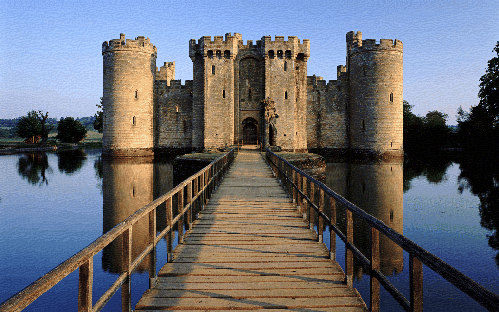
Train step: 1500
CPU times: user 3min 34s, sys: 1min 55s, total: 5min 30s
Wall time: 5min 40s
显示风格迁移图像生成过程的GIF图像
# 读取GIF动画文件
animation_path = 'animation.gif'

# 使用Image函数显示GIF动画
Image(filename=animation_path)
8 总变分损失
此实现只是一个基础版本,它的一个缺点是它会产生大量的高频误差。 我们可以直接通过正则化图像的高频分量来减少这些高频误差。 在风格转移中,这通常被称为总变分损失:
def high_pass_x_y(image):
  # 图像在 x 和 y 方向上的高通变化
  x_var = image[:, :, 1:, :] - image[:, :, :-1, :]
  y_var = image[:, 1:, :, :] - image[:, :-1, :, :]

  return x_var, y_var
x_deltas, y_deltas = high_pass_x_y(content_image)

plt.figure(figsize=(14, 10))
plt.subplot(2, 2, 1)
# 关闭坐标轴显示
plt.axis('off')
imshow(clip_0_1(2*y_deltas+0.5), "Horizontal Deltas: Original")

plt.subplot(2, 2, 2)
# 关闭坐标轴显示
plt.axis('off')
imshow(clip_0_1(2*x_deltas+0.5), "Vertical Deltas: Original")

x_deltas, y_deltas = high_pass_x_y(image)

plt.subplot(2, 2, 3)
# 关闭坐标轴显示
plt.axis('off')
imshow(clip_0_1(2*y_deltas+0.5), "Horizontal Deltas: Styled")

plt.subplot(2, 2, 4)
# 关闭坐标轴显示
plt.axis('off')
imshow(clip_0_1(2*x_deltas+0.5), "Vertical Deltas: Styled")
对原始图像和样式化图像进行高通变化的可视化展示。
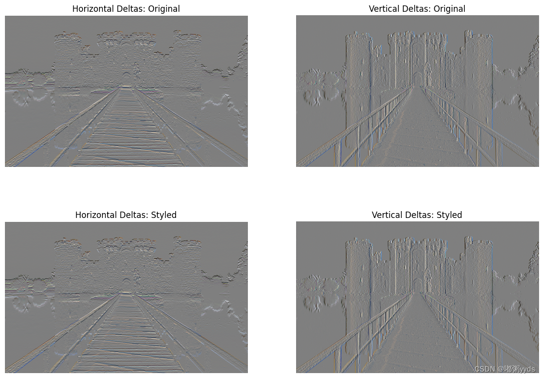
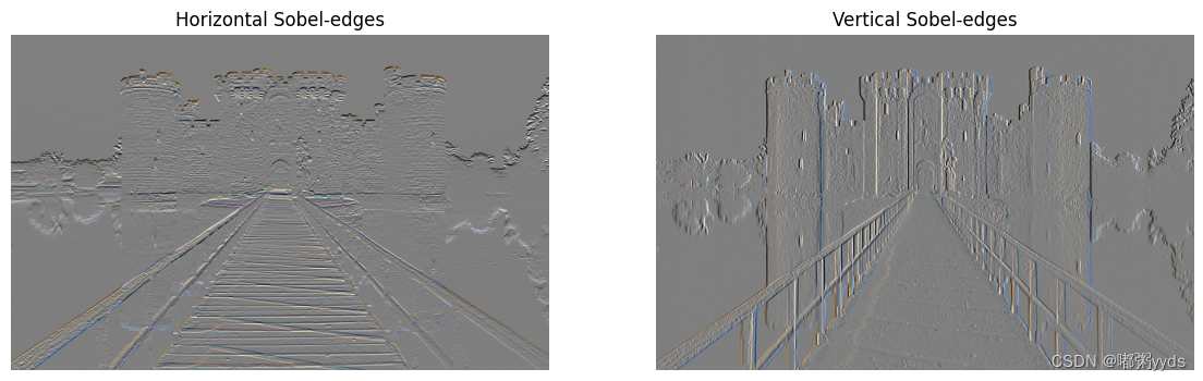
这显示了高频分量如何增加。而且,本质上高频分量是一个边缘检测器。 我们可以从 Sobel 边缘检测器获得类似的输出,例如:
plt.figure(figsize=(14, 10))

sobel = tf.image.sobel_edges(content_image)
plt.subplot(1, 2, 1)
# 关闭坐标轴显示
plt.axis('off')
imshow(clip_0_1(sobel[..., 0]/4+0.5), "Horizontal Sobel-edges")
plt.subplot(1, 2, 2)
# 关闭坐标轴显示
plt.axis('off')
imshow(clip_0_1(sobel[..., 1]/4+0.5), "Vertical Sobel-edges")
与此相关的正则化损失是这些值的平方和:
def total_variation_loss(image):
  x_deltas, y_deltas = high_pass_x_y(image)
  return tf.reduce_sum(tf.abs(x_deltas)) + tf.reduce_sum(tf.abs(y_deltas))
total_variation_loss(image).numpy() # 118979.87
这展示了它的作用。但是没有必要自己去实现它,因为 TensorFlow 包括一个标准的实现:
tf.image.total_variation(image).numpy() # array([118979.87], dtype=float32)
9 重新优化
选择 total_variation_loss 的权重:
total_variation_weight=30

@tf.function()
def train_step(image):
  with tf.GradientTape() as tape:
    outputs = extractor(image)
    loss = style_content_loss(outputs)
    loss += total_variation_weight * tf.image.total_variation(image)

  grad = tape.gradient(loss, image)
  opt.apply_gradients([(grad, image)])
  image.assign(clip_0_1(image))

# 重新初始化优化的变量
image = tf.Variable(content_image)
%%time

epochs = 15
steps_per_epoch = 100

enhance_images = []

step = 0
for n in range(epochs):
  for m in range(steps_per_epoch):
    step += 1
    train_step(image)
    print(".", end='', flush=True)
    if m % interval[n] == 0:
      # 将图像添加到列表中
      enhance_images.append(tensor_to_image(image))
  display.clear_output(wait=True)
  display.display(tensor_to_image(image))
  print("Train step: {}".format(step))
# 将图像列表保存为 GIF 动画
imageio.mimsave('enhance_animation.gif', enhance_images, fps=10)
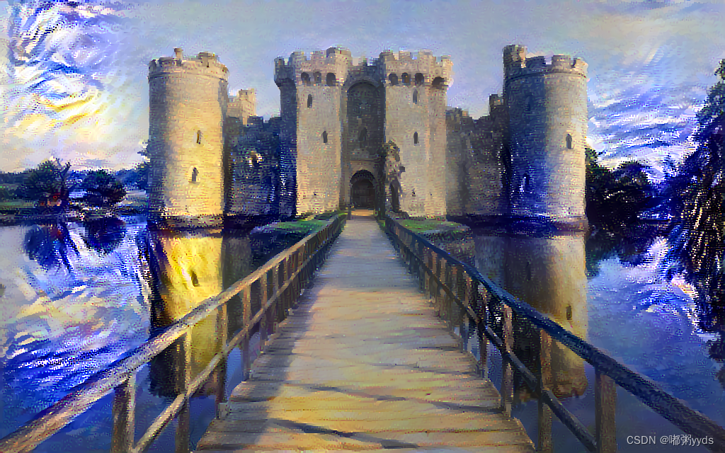
Train step: 1500
CPU times: user 3min 30s, sys: 1min 58s, total: 5min 28s
Wall time: 5min 45s
显示优化后的风格迁移图像生成过程的GIF图像
# 读取GIF动画文件
animation_path = 'enhance_animation.gif'

# 使用Image函数显示GIF动画
Image(filename=animation_path)