【生物信息学】Notears Linear算法在线性结构方程模型中的因果关系估计

Notears Linear算法是一种用于估计线性结构方程模型中因果关系的有效方法。它通过最小化损失函数来寻找最优的权重矩阵，使得该矩阵能够描述变量之间的因果关系。该算法具有以下优点：

高效性：Notears Linear算法使用了一种基于优化的方法，可以高效地估计因果关系。该算法的复杂度取决于变量的数量和观测样本的大小，但通常具有较低的计算复杂度。

线性模型适用性：Notears Linear算法适用于线性结构方程模型，可以有效地处理线性因果关系。对于非线性关系，该算法可能不适用。

约束项的引入：Notears Linear算法引入了约束项来确保估计的图是无环的，从而建立了因果关系的因果性。这有助于提高估计结果的解释性和可靠性。

二、实验环境

本系列实验使用了PyTorch深度学习框架，相关操作如下（基于深度学习系列文章的环境）：

1. 配置虚拟环境

深度学习系列文章的环境

conda create -n DL python=3.7

conda activate DL

pip install torch==1.8.1+cu102 torchvision==0.9.1+cu102 torchaudio==0.8.1 -f https://download.pytorch.org/whl/torch_stable.html

conda install matplotlib

conda install scikit-learn

新增加

conda install pandas

conda install seaborn

conda install networkx

conda install statsmodels

pip install pyHSICLasso

注：本人的实验环境按照上述顺序安装各种库，若想尝试一起安装（天知道会不会出问题）

2. 库版本介绍

软件包	本实验版本	目前最新版
matplotlib	3.5.3	3.8.0
numpy	1.21.6	1.26.0
python	3.7.16
scikit-learn	0.22.1	1.3.0
torch	1.8.1+cu102	2.0.1
torchaudio	0.8.1	2.0.2
torchvision	0.9.1+cu102	0.15.2

新增

networkx	2.6.3	3.1
pandas	1.2.3	2.1.1
pyHSICLasso	1.4.2	1.4.2
seaborn	0.12.2	0.13.0
statsmodels	0.13.5	0.14.0

3. IDE

建议使用Pycharm（其中，pyHSICLasso库在VScode出错，尚未找到解决办法……）

内部函数

三、实验内容

0. 导入必要的工具

import numpy as np
import scipy.linalg as slin
import scipy.optimize as sopt
import random

import networkx as nx
import matplotlib.pyplot as plt

1. set_random_seed

def set_random_seed(seed=1):
    random.seed(seed)
    np.random.seed(seed)

用于设置随机种子，以确保结果的可重复性。

2. notears_linear

def notears_linear(X, lambda1=0.08, max_iter=100, h_tol=1e-8, rho_max=1e+16, w_threshold=0.3):

a. 输入参数

X：输入的数据矩阵，形状为 (n, d)，其中 n 是样本数量，d 是特征维度。
lambda1：L1 正则化项的权重，默认为 0.08。
max_iter：最大迭代次数，默认为 100。
h_tol：停止迭代的目标误差容限，默认为 1e-8。
rho_max：最大惩罚参数，默认为 1e+16。
w_threshold：权重的阈值，用于稀疏化估计的结果，默认为 0.3。

函数内部定义了几个辅助函数，包括

b. 内部函数`_adj`

   def _adj(w):
        return w.reshape([d, d])

将扁平化的权重参数w转换为方阵形式的权重矩阵W。

`c.` 内部函数`_loss`

    def _loss(W):
        X_ = X @ W
        R = X - X_
        loss = 0.5 / X.shape[0] * (R ** 2).sum() + lambda1 * W.sum()  # Form 2
        G_loss = - 1.0 / X.shape[0] * X.T @ R + lambda1

        return loss, G_loss

计算损失函数和其梯度。
- 损失函数包括两部分：数据拟合项和正则化项。
- 梯度表示损失函数对权重矩阵的导数。

`d.`内部函数`_h`

    def _h(W):
        E = slin.expm(W * W)
        h = np.trace(E) - d
        G_h = E.T * W * 2  # Form 6
        return h, G_h

计算另一个约束项和其梯度。
- 约束项用于确保估计的图是无环的。
- 梯度表示约束项对权重矩阵的导数。

`e.`内部函数`_func`

    def _func(w):
        W = _adj(w)
        loss, G_loss = _loss(W)
        h, G_h = _h(W)
        obj = loss + 0.5 * rho * h * h + alpha * h  # Form 11
        G_smooth = G_loss + (rho * h + alpha) * G_h  # G of Form 11
        g_obj = G_smooth.reshape(-1, )
        return obj, g_obj

计算完整的目标函数和其梯度。
- 目标函数包括损失函数、约束项和正则化项。
- 梯度表示目标函数对权重参数的导数。

f. 函数主体部分

    n, d = X.shape
    w_est, rho, alpha, h = np.zeros(d * d), 1.0, 0.0, np.inf
    bnds = [(0, 0) if i == j else (0, None) for i in range(d) for j in range(d)]
    X = X - np.mean(X, axis=0)
    for _ in range(max_iter):
        w_new, h_new = None, None
        while rho < rho_max:
            sol = sopt.minimize(_func, w_est, jac=True, bounds=bnds)
            w_new = sol.x
            h_new, _ = _h(_adj(w_new))
            if h_new > 0.25 * h:  # h下降不够快时 提高h的权重
                rho *= 10
            else:
                break
        w_est, h = w_new, h_new
        alpha += rho * h
        if h <= h_tol or rho >= rho_max:
            break
    W_est = _adj(w_est)
    W_est[np.abs(W_est) < w_threshold] = 0
    return W_est

初始化变量
- 获取输入数据矩阵的维度并初始化一些变量。
- 对输入数据矩阵进行中心化处理。
循环迭代
- 在每次迭代中，通过调用 scipy.optimize.minimize 函数来寻找最优的模型参数估计。
- 在寻找最优解的过程中，通过调整惩罚参数 rho 的值来控制模型结构的稀疏性。
- 在迭代过程中，根据目标函数的值和约束条件的变化情况来动态调整 rho 的值。
- 当达到停止条件（目标误差小于容限或者惩罚参数 rho 达到最大值）时，停止迭代。
阈值处理：将权重矩阵中绝对值小于给定阈值的元素置为零。
返回估计得到的模型参数矩阵W_est。

3. 主程序

if __name__ == '__main__':
    set_random_seed()

    X = np.loadtxt('Notears_X.csv', delimiter=',')
    W_est = notears_linear(X)

    print("W_est")
    print(W_est)

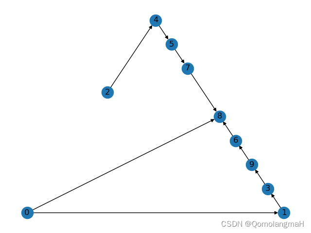
    G_nx = nx.DiGraph(W_est)
    print(nx.is_directed_acyclic_graph(G_nx))

    nx.draw_planar(G_nx, with_labels=True)
    plt.show()

设置随机种子。
从文件 "Notears_X.csv" 中加载数据矩阵 X。

调用 notears_linear 函数，估计线性结构方程模型的参数，得到估计的模型参数矩阵 W_est。
打印输出估计的模型参数矩阵 W_est。
根据估计的模型参数矩阵 W_est 创建一个有向图 G_nx。
判断图 G_nx 是否是有向无环图（DAG）。
绘制图 G_nx 的平面布局，并显示图形。

数据部分展示

6.24E-01	9.07E-01	7.77E-01	1.58E+00	#######	#######	5.62E+00	#######	#######	7.16E+00
7.50E-01	7.33E-01	#######	7.01E-03	#######	#######	3.93E-01	#######	2.40E+00	#######
3.77E-01	7.12E-01	1.71E-01	1.58E-01	1.08E+00	1.73E+00	#######	3.05E+00	4.09E+00	#######
1.39E-01	1.10E+00	7.96E-01	1.67E+00	2.94E-01	#######	4.86E+00	#######	#######	7.24E+00
#######	#######	#######	#######	#######	9.83E-01	#######	3.42E+00	4.28E+00	#######
#######	#######	8.44E-01	5.92E-01	9.75E-02	#######	#######	8.99E-01	#######	1.18E+00
#######	1.68E-01	#######	#######	1.50E+00	3.22E+00	#######	3.14E+00	4.26E+00	#######
#######	#######	2.18E-01	#######	1.18E+00	2.19E+00	#######	1.41E+00	9.86E-01	#######
1.85E-01	3.48E-02	3.65E-01	#######	3.91E-01	1.97E+00	#######	4.16E+00	4.85E+00	#######
#######	#######	#######	#######	3.01E-01	7.11E-01	2.77E-02	#######	#######	#######

绘制图

n. 代码整合

import numpy as np
import scipy.linalg as slin
import scipy.optimize as sopt
import random

import networkx as nx
import matplotlib.pyplot as plt


def set_random_seed(seed=1):
    random.seed(seed)
    np.random.seed(seed)


def notears_linear(X, lambda1=0.08, max_iter=100, h_tol=1e-8, rho_max=1e+16, w_threshold=0.3):

    def _adj(w):
        return w.reshape([d, d])

    def _loss(W):
        X_ = X @ W
        R = X - X_
        loss = 0.5 / X.shape[0] * (R ** 2).sum() + lambda1 * W.sum()  # Form 2
        G_loss = - 1.0 / X.shape[0] * X.T @ R + lambda1

        return loss, G_loss

    def _h(W):
        E = slin.expm(W * W)
        h = np.trace(E) - d
        G_h = E.T * W * 2  # Form 6
        return h, G_h


    def _func(w):
        W = _adj(w)
        loss, G_loss = _loss(W)
        h, G_h = _h(W)
        obj = loss + 0.5 * rho * h * h + alpha * h  # Form 11
        G_smooth = G_loss + (rho * h + alpha) * G_h  # G of Form 11
        g_obj = G_smooth.reshape(-1, )
        return obj, g_obj

    n, d = X.shape
    w_est, rho, alpha, h = np.zeros(d * d), 1.0, 0.0, np.inf
    bnds = [(0, 0) if i == j else (0, None) for i in range(d) for j in range(d)]
    X = X - np.mean(X, axis=0)
    for _ in range(max_iter):
        w_new, h_new = None, None
        while rho < rho_max:
            sol = sopt.minimize(_func, w_est, jac=True, bounds=bnds)
            w_new = sol.x
            h_new, _ = _h(_adj(w_new))
            if h_new > 0.25 * h:  # h下降不够快时 提高h的权重
                rho *= 10
            else:
                break
        w_est, h = w_new, h_new
        alpha += rho * h
        if h <= h_tol or rho >= rho_max:
            break
    W_est = _adj(w_est)
    W_est[np.abs(W_est) < w_threshold] = 0
    return W_est


if __name__ == '__main__':
    set_random_seed()

    X = np.loadtxt('Notears_X.csv', delimiter=',')
    W_est = notears_linear(X)

    print("W_est")
    print(W_est)

    G_nx = nx.DiGraph(W_est)
    print(nx.is_directed_acyclic_graph(G_nx))

    nx.draw_planar(G_nx, with_labels=True)
    plt.show()

    # edges, weights = zip(*nx.get_edge_attributes(G_nx, 'weight').items())
    # pos = nx.spring_layout(G_nx)
    # nx.draw(G_nx, pos, node_color='b', edgelist=edges, edge_color=weights, width=5, with_labels=True, edge_cmap=plt.cm.Blues)
    # plt.show()