目录
1. R Studio界面
设置工作界面:
Note:R语言的排序从1开始,与python从0开始的做法不一样
右下角界面: 点File然后进入到你需要到的界面-然后点带齿轮的More - Set as working directory.

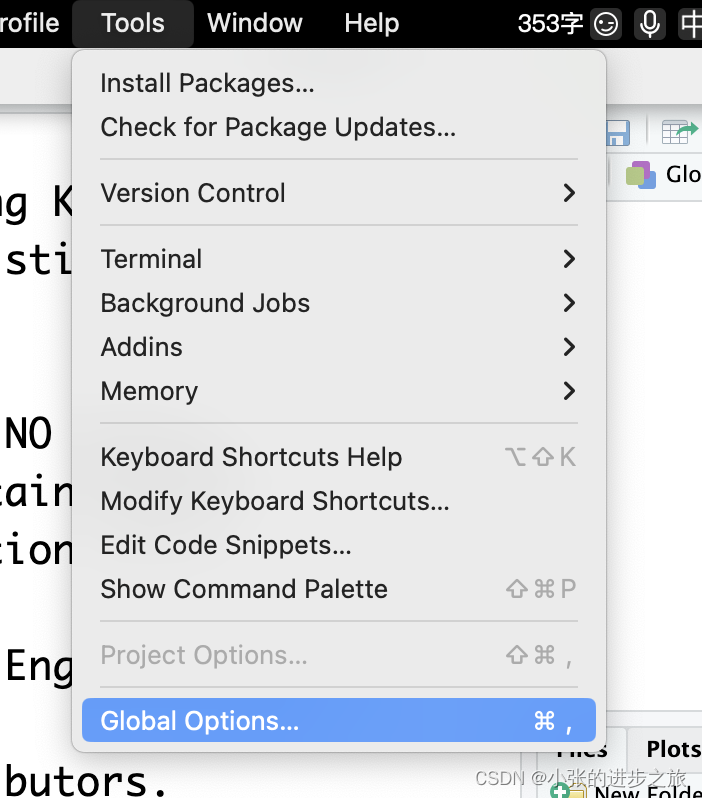
如果不想要每次都打开选择这么多文件夹,可以选择使用Tools-Global setting- Deafault working directory.
2. 数据处理
2.1 数据类型
- 向量 (vector)
- 列表 (list)
- 矩阵 (matrix)
- 数组 (Array)
- 因子 (Factor)
- 数据框 (Data Frame)
除了因子以外,其他数据类型在python中都有,在这里不进行重复,因子是一个比较新的数据类型: 详细的解释可见:R 因子 | 菜鸟教程
总的来说就是类似list的变量会带一个class,用于对数据进行归类。 以下为几个例子:
gender <- factor(c("MALE", "FEMALE", "MALE"))
gender
得到的结果如下:
[1] MALE FEMALE MALE
Levels: FEMALE MALE
也就是除了正常的数据以外,会带一个levels, 包含他们的划分
blood <- factor(c("O", "AB", "A"),
                levels = c("A", "B", "AB", "O"))
blood
[1] O AB A
Levels: A B AB O
再比如说以上的在这个例子中, 虽然在blood这个因子中不包含B这个类型, 但是总的分类中是有的。
也可以用于排序:
# add ordered factor
symptoms <- factor(c("SEVERE", "MILD", "MODERATE"),
                   levels = c("MILD", "MODERATE", "SEVERE"),
                   ordered = TRUE)
symptoms

# check for symptoms greater than moderate
symptoms > "MODERATE"
[1] MALE FEMALE MALE Levels: FEMALE MALE
[1] TRUE FALSE FALSE

2.2 数据的基本处理
1. 选取某一列数据:
subject1$temperature $符号代表某一列的数据
2. 根据名字选取几列
# get several list items by specifying a vector of names

subject1[c("temperature", "flu_status")]
3. 根据序号选取几列
## access a list like a vector # get values 2 and 3

subject1[2:3]
4. 新建一个dataframe
# create a data frame from medical patient data
pt_data <- data.frame(subject_name, temperature, flu_status, gender, blood, symptoms)
5. 截取行或者列的数据
# column 1,
all rows pt_data[, 1]
# row 1, all columns
pt_data[1, ]
# all rows and all columns
pt_data[ , ]
6. 建立不同维度的矩阵
# create a 2x3 matrix
m <- matrix(c(1, 2, 3, 4, 5, 6), nrow = 2)
# create a 3x2 matrix
m <- matrix(c(1, 2, 3, 4, 5, 6), ncol = 2)
2.3 管理数据
# show all data structures in memory 展示所有的数据
ls()
# remove the m and subject1 objects 清除数据
rm(m, subject1)
ls()
rm(list=ls())
3. 导入数据
3.1导入csv数据
可以使用代码进行数据的导入
# reading a CSV file
pt_data <- read.csv("pt_data.csv")
# reading a CSV file and converting all character columns to factors
pt_data <- read.csv("pt_data.csv", stringsAsFactors = TRUE)
也可以直接使用右上角的import dataset来进行数据的导入
3.2 得到数据的结构
# get structure of used car data
str(usedcars)
3.3 总结数据
# summarize numeric variables  对数据进行总结
summary(usedcars$year)
summary(usedcars[c("price", "mileage")])
Min. 1st Qu. Median Mean 3rd Qu. Max. 2000 2008 2009 2009 2010 2012
# calculate the mean income
(36000 + 44000 + 56000) / 3
mean(c(36000, 44000, 56000))

# the median income
median(c(36000, 44000, 56000))

# the min/max of used car prices
range(usedcars$price)

# the difference of the range
diff(range(usedcars$price))

# IQR for used car prices 四分位距 (Interquartile range)
IQR(usedcars$price)

# use quantile to calculate five-number summary
quantile(usedcars$price)

# the 99th percentile
quantile(usedcars$price, probs = c(0.01, 0.99))
绘图:
# quintiles
quantile(usedcars$price, seq(from = 0, to = 1, by = 0.20))

# boxplot of used car prices and mileage
boxplot(usedcars$price, main = "Boxplot of Used Car Prices",
      ylab = "Price ($)")

boxplot(usedcars$mileage, main="Boxplot of Used Car Mileage",
      ylab = "Odometer (mi.)")

# histograms of used car prices and mileage
hist(usedcars$price, main = "Histogram of Used Car Prices",
     xlab = "Price ($)")

hist(usedcars$mileage, main = "Histogram of Used Car Mileage",
     xlab = "Odometer (mi.)")
对数据的variance和方差进行探究
# variance and standard deviation of the used car data
var(usedcars$price)
sd(usedcars$price)
var(usedcars$mileage)
sd(usedcars$mileage)

## Exploring numeric variables -----

# one-way tables for the used car data
table(usedcars$year)
table(usedcars$model)
table(usedcars$color)
table是对数据的频数进行统计:如下图所示:
2000 2001 2002 2003 2004 2005 2006 2007 2008 2009 2010 2011
3 1 1 1 3 2 6 11 14 42 49 16 2012 1
# compute table proportions
model_table <- table(usedcars$model)
prop.table(model_table) #对频数的百分比进行计算

# round the data
color_table <- table(usedcars$color)
color_pct <- prop.table(color_table) * 100
round(color_pct, digits = 1)