隐马尔可夫模型(HMM)是可用于标注问题的统计模型。关于HMM通常包含三类问题:1.概率计算 2.参数学习 3.预测状态。本博客简单罗列下HMM的知识点,给出代码。详细地参考李航《统计学习方法》。
模型简介
HMM描述先由隐藏的马尔可夫链生成状态序列,各个状态序列生成一个观测,组合成最终的观测序列。故整个模型包含三个要素:
1. 初始状态概率向量:生成第一个状态的概率
2. 状态转移概率矩阵:当前状态转移到下一个状态的概率矩阵
3. 观测生成概率矩阵:每个状态生成各个观测的概率
概率计算问题
给定模型,求解观测序列出现的概率。直接求解概率的计算十分复杂,通常采用递推的方法求解,即从部分序列到整体序列。可以从前往后递推,也可从后往前递推。
前向算法
前向概率:到时刻t的部分观测序列的时刻t状态为
的概率。
时刻t-1的每个可能状态乘以状态转移概率,和再乘以观测生成概率即为时刻t的前向概率。
后向概率:对于时刻t+1到T的部分序列,在时刻t的状态为
的概率。
时刻t+1的每个可能状态乘以观测生成概率,再乘以状态转移概率, 和即为时刻t的前向概率。
参数学习
隐马尔可夫模型中”状态”时隐藏的,是一个典型的含有隐藏变量的模型,故需要使用EM算法来学习模型参数。EM算法应用到HMM模型中时称为Baum-Welch算法。
预测状态
状态序列是比较长且可能性非常多的,首先想到将问题规模缩小。而在隐马尔可夫模型中,当前状态是依赖于前一个状态的,那么规模缩小后,子问题之间必定是相关的,应当采用动态规划的算法,即Viterbi算法。该算法将状态序列视为一条路径,那么路径的长度就是状态转移概率乘以观测生成概率,再求和。问题变为求解最长路径。如图所示: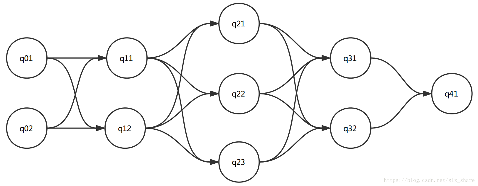
- 子问题结构:从0时刻到时刻t且状态为i的所有路径中的最长路径。定义最长路径长度为
- 递推式:时刻t+1且状态为i的最长路径长度必然是到时刻t的最长路径长度加上t到t+1的最长路径。
- 构造最优解:在求解子问题的过程中,存储上一个时刻的状态。最后递归构建最优解。
代码
"""
隐马尔科夫模型
三类问题:1.概率计算 2.学习问题(参数估计) 3.预测问题(状态序列的预测)
"""
import numpy as np
from itertools import accumulate


class GenData:
    """
    根据隐马尔科夫模型生成相应的观测数据
    """

    def __init__(self, hmm, n_sample):
        self.hmm = hmm
        self.n_sample = n_sample

    def _locate(self, prob_arr):
        # 给定概率向量,返回状态
        seed = np.random.rand(1)
        for state, cdf in enumerate(accumulate(prob_arr)):
            if seed <= cdf:
                return state
        return

    def init_state(self):
        # 根据初始状态概率向量,生成初始状态
        return self._locate(self.hmm.S)

    def state_trans(self, current_state):
        # 转移状态
        return self._locate(self.hmm.A[current_state])

    def gen_obs(self, current_state):
        # 生成观测
        return self._locate(self.hmm.B[current_state])

    def gen_data(self):
        # 根据模型产生观测数据
        current_state = self.init_state()
        start_obs = self.gen_obs(current_state)
        state = [current_state]
        obs = [start_obs]
        n = 0
        while n < self.n_sample - 1:
            n += 1
            current_state = self.state_trans(current_state)
            state.append(current_state)
            obs.append(self.gen_obs(current_state))
        return state, obs


class HMM:
    def __init__(self, n_state, n_obs, S=None, A=None, B=None):
        self.n_state = n_state  # 状态的个数n
        self.n_obs = n_obs  # 观测的种类数m
        self.S = S  # 1*n, 初始状态概率向量
        self.A = A  # n*n, 状态转移概率矩阵
        self.B = B  # n*m, 观测生成概率矩阵


def _alpha(hmm, obs, t):
    # 计算时刻t各个状态的前向概率
    b = hmm.B[:, obs[0]]
    alpha = np.array([hmm.S * b])  # n*1
    for i in range(1, t + 1):
        alpha = (alpha @ hmm.A) * np.array([hmm.B[:, obs[i]]])
    return alpha[0]


def forward_prob(hmm, obs):
    # 前向算法计算最终生成观测序列的概率, 即各个状态下概率之和
    alpha = _alpha(hmm, obs, len(obs) - 1)
    return np.sum(alpha)


def _beta(hmm, obs, t):
    # 计算时刻t各个状态的后向概率
    beta = np.ones(hmm.n_state)
    for i in reversed(range(t + 1, len(obs))):
        beta = np.sum(hmm.A * hmm.B[:, obs[i]] * beta, axis=1)
    return beta


def backward_prob(hmm, obs):
    # 后向算法计算生成观测序列的概率
    beta = _beta(hmm, obs, 0)
    return np.sum(hmm.S * hmm.B[:, obs[0]] * beta)


def fb_prob(hmm, obs, t=None):
    # 将前向和后向合并
    if t is None:
        t = 0
    res = _alpha(hmm, obs, t) * _beta(hmm, obs, t)
    return res.sum()


def _gamma(hmm, obs, t):
    # 计算时刻t处于各个状态的概率
    alpha = _alpha(hmm, obs, t)
    beta = _beta(hmm, obs, t)
    prob = alpha * beta
    return prob / prob.sum()


def point_prob(hmm, obs, t, i):
    # 计算时刻t处于状态i的概率
    prob = _gamma(hmm, obs, t)
    return prob[i]


def _xi(hmm, obs, t):
    alpha = np.mat(_alpha(hmm, obs, t))
    beta_p = _beta(hmm, obs, t + 1)
    obs_prob = hmm.B[:, obs[t + 1]]
    obs_beta = np.mat(obs_prob * beta_p)
    alpha_obs_beta = np.asarray(alpha.T * obs_beta)
    xi = alpha_obs_beta * hmm.A
    return xi / xi.sum()


def fit(hmm, obs_data, maxstep=100):
    # 利用Baum-Welch算法学习
    hmm.A = np.ones((hmm.n_state, hmm.n_state)) / hmm.n_state
    hmm.B = np.ones((hmm.n_state, hmm.n_obs)) / hmm.n_obs
    hmm.S = np.random.sample(hmm.n_state)  # 初始状态概率矩阵(向量),的初始化必须随机状态,否则容易陷入局部最优
    hmm.S = hmm.S / hmm.S.sum()
    step = 0
    while step < maxstep:
        xi = np.zeros_like(hmm.A)
        gamma = np.zeros_like(hmm.S)
        B = np.zeros_like(hmm.B)
        S = _gamma(hmm, obs_data, 0)
        for t in range(len(obs_data) - 1):
            tmp_gamma = _gamma(hmm, obs_data, t)
            gamma += tmp_gamma
            xi += _xi(hmm, obs_data, t)
            B[:, obs_data[t]] += tmp_gamma

        # 更新 A
        for i in range(hmm.n_state):
            hmm.A[i] = xi[i] / gamma[i]
        # 更新 B
        tmp_gamma_end = _gamma(hmm, obs_data, len(obs_data) - 1)
        gamma += tmp_gamma_end
        B[:, obs_data[-1]] += tmp_gamma_end
        for i in range(hmm.n_state):
            hmm.B[i] = B[i] / gamma[i]
        # 更新 S
        hmm.S = S
        step += 1
    return hmm


def predict(hmm, obs):
    # 采用Viterbi算法预测状态序列
    N = len(obs)
    nodes_graph = np.zeros((hmm.n_state, N), dtype=int)  # 存储时刻t且状态为i时, 前一个时刻t-1的状态,用于构建最终的状态序列
    delta = hmm.S * hmm.B[:, obs[0]]  # 存储到t时刻,且此刻状态为i的最大概率
    nodes_graph[:, 0] = range(hmm.n_state)

    for t in range(1, N):
        new_delta = []
        for i in range(hmm.n_state):
            temp = [hmm.A[j, i] * d for j, d in enumerate(delta)]  # 当前状态为i时, 选取最优的前一时刻状态
            max_d = max(temp)
            new_delta.append(max_d * hmm.B[i, obs[t]])
            nodes_graph[i, t] = temp.index(max_d)
        delta = new_delta

    current_state = np.argmax(nodes_graph[:, -1])
    path = []
    t = N
    while t > 0:
        path.append(current_state)
        current_state = nodes_graph[current_state, t - 1]
        t -= 1
    return list(reversed(path))


if __name__ == '__main__':
    # S = np.array([0.2, 0.4, 0.4])
    # A = np.array([[0.5, 0.2, 0.3], [0.3, 0.5, 0.2], [0.2, 0.3, 0.5]])
    # B = np.array([[0.5, 0.2, 0.3], [0.4, 0.2, 0.4], [0.6, 0.3, 0.1]])
    # hmm_real = HMM(3, 3, S, A, B)
    # g = GenData(hmm_real, 500)
    # state, obs = g.gen_data()
    # 检测生成的数据
    # state, obs = np.array(state), np.array(obs)
    # ind = np.where(state==2)[0]
    # from collections import Counter
    # obs_ind = obs[ind]
    # c1 = Counter(obs_ind)
    # n = sum(c1.values())
    # for o, val in c.items():
    #     print(o, val/n)
    # ind_next = ind + 1
    # ind_out = np.where(ind_next==1000)
    # ind_next = np.delete(ind_next, ind_out)
    # state_next = state[ind_next]
    # c2 = Counter(state_next)
    # n = sum(c2.values())
    # for s, val in c2.items():
    #     print(s, val/n)

    # 预测
    S = np.array([0.5, 0.5])
    A = np.array([[0.8, 1], [0.8, 0.8]])
    B = np.array([[0.2, 0.0, 0.8], [0, 0.8, 0.2]])
    hmm = HMM(2, 3, S, A, B)
    g = GenData(hmm, 200)
    state, obs = g.gen_data()
    print(obs)
    path = predict(hmm, obs)
    score = sum([int(i == j) for i, j in zip(state, path)])
    print(score / len(path))


    # 学习
    # import matplotlib.pyplot as plt
    #
    #
    # def triangle_data(n_sample):
    #     # 生成三角波形状的序列
    #     data = []
    #     for x in range(n_sample):
    #         x = x % 6
    #         if x <= 3:
    #             data.append(x)
    #         else:
    #             data.append(6 - x)
    #     return data
    #
    #
    # hmm = HMM(10, 4)
    # data = triangle_data(30)
    # hmm = fit(hmm, data)
    # g = GenData(hmm, 30)
    # state, obs = g.gen_data()
    #
    # x = [i for i in range(30)]
    # plt.scatter(x, obs, marker='*', color='r')
    # plt.plot(x, data, color='g')
    # plt.show()
我的GitHub
注:如有不当之处,请指正。