数据规整化:清理、转换、合并、重塑 第7章
合并数据集
pandas.merge可以根据一个或多个键将不同DataFrame中的行连接起来。
pandas.concat可以沿着一条轴将多个对象堆叠到一起
实例方法combine_first可以将重复数据编接在一起,类似于数据库中的全外连接
数据库风格的DataFrame合并
数据集的合并(merge)或连接(join)运算是通过一个或多个键将行链接起来的。这些运算关系是关系型数据库的核心
import pandas as pd
from pandas import DataFrame,Series
df1=DataFrame({'key':['b','b','a','c','a','a','b'],'data1':range(7)})
df2=DataFrame({'key':['a','b','d'],'data2':range(3)})
df1
|
data1 |
key |
| 0 |
0 |
b |
| 1 |
1 |
b |
| 2 |
2 |
a |
| 3 |
3 |
c |
| 4 |
4 |
a |
| 5 |
5 |
a |
| 6 |
6 |
b |
df2
|
data2 |
key |
| 0 |
0 |
a |
| 1 |
1 |
b |
| 2 |
2 |
d |
pd.merge(df1,df2)
|
data1 |
key |
data2 |
| 0 |
0 |
b |
1 |
| 1 |
1 |
b |
1 |
| 2 |
6 |
b |
1 |
| 3 |
2 |
a |
0 |
| 4 |
4 |
a |
0 |
| 5 |
5 |
a |
0 |
pd.merge(df1,df2,on='key')
|
data1 |
key |
data2 |
| 0 |
0 |
b |
1 |
| 1 |
1 |
b |
1 |
| 2 |
6 |
b |
1 |
| 3 |
2 |
a |
0 |
| 4 |
4 |
a |
0 |
| 5 |
5 |
a |
0 |
df3=DataFrame({'lkey':['b','b','a','c','a','a','b'],'data1':range(7)})
df4=DataFrame({'rkey':['a','b','d'],'data2':range(3)})
pd.merge(df3,df4,left_on='lkey',right_on='rkey')
|
data1 |
lkey |
data2 |
rkey |
| 0 |
0 |
b |
1 |
b |
| 1 |
1 |
b |
1 |
b |
| 2 |
6 |
b |
1 |
b |
| 3 |
2 |
a |
0 |
a |
| 4 |
4 |
a |
0 |
a |
| 5 |
5 |
a |
0 |
a |
pd.merge(df1,df2,how='outer')
|
data1 |
key |
data2 |
| 0 |
0.0 |
b |
1.0 |
| 1 |
1.0 |
b |
1.0 |
| 2 |
6.0 |
b |
1.0 |
| 3 |
2.0 |
a |
0.0 |
| 4 |
4.0 |
a |
0.0 |
| 5 |
5.0 |
a |
0.0 |
| 6 |
3.0 |
c |
NaN |
| 7 |
NaN |
d |
2.0 |
df1=DataFrame({'key':['b','b','a','c','a','b'],'data1':range(6)})
df2=DataFrame({'key':['a','b','a','b','d'],'data2':range(5)})
df1
|
data1 |
key |
| 0 |
0 |
b |
| 1 |
1 |
b |
| 2 |
2 |
a |
| 3 |
3 |
c |
| 4 |
4 |
a |
| 5 |
5 |
b |
df2
|
data2 |
key |
| 0 |
0 |
a |
| 1 |
1 |
b |
| 2 |
2 |
a |
| 3 |
3 |
b |
| 4 |
4 |
d |
pd.merge(df1,df2,on='key',how='left')
|
data1 |
key |
data2 |
| 0 |
0 |
b |
1.0 |
| 1 |
0 |
b |
3.0 |
| 2 |
1 |
b |
1.0 |
| 3 |
1 |
b |
3.0 |
| 4 |
2 |
a |
0.0 |
| 5 |
2 |
a |
2.0 |
| 6 |
3 |
c |
NaN |
| 7 |
4 |
a |
0.0 |
| 8 |
4 |
a |
2.0 |
| 9 |
5 |
b |
1.0 |
| 10 |
5 |
b |
3.0 |
pd.merge(df1,df2,how='inner')
|
data1 |
key |
data2 |
| 0 |
0 |
b |
1 |
| 1 |
0 |
b |
3 |
| 2 |
1 |
b |
1 |
| 3 |
1 |
b |
3 |
| 4 |
5 |
b |
1 |
| 5 |
5 |
b |
3 |
| 6 |
2 |
a |
0 |
| 7 |
2 |
a |
2 |
| 8 |
4 |
a |
0 |
| 9 |
4 |
a |
2 |
left=DataFrame({'key1':['foo','foo','bar'],'key2':['one','two','one']
,'lval':[1,2,3]})
right=DataFrame({'key1':['foo','foo','bar','bar'],'key2':['one','one','one','two']
,'rval':[4,5,6,7]})
pd.merge(left,right,on=['key1','key2'],how='outer')
|
key1 |
key2 |
lval |
rval |
| 0 |
foo |
one |
1.0 |
4.0 |
| 1 |
foo |
one |
1.0 |
5.0 |
| 2 |
foo |
two |
2.0 |
NaN |
| 3 |
bar |
one |
3.0 |
6.0 |
| 4 |
bar |
two |
NaN |
7.0 |
pd.merge(left,right,on='key1')
|
key1 |
key2_x |
lval |
key2_y |
rval |
| 0 |
foo |
one |
1 |
one |
4 |
| 1 |
foo |
one |
1 |
one |
5 |
| 2 |
foo |
two |
2 |
one |
4 |
| 3 |
foo |
two |
2 |
one |
5 |
| 4 |
bar |
one |
3 |
one |
6 |
| 5 |
bar |
one |
3 |
two |
7 |
pd.merge(left,right,on='key1',suffixes=('_left','_right'))
|
key1 |
key2_left |
lval |
key2_right |
rval |
| 0 |
foo |
one |
1 |
one |
4 |
| 1 |
foo |
one |
1 |
one |
5 |
| 2 |
foo |
two |
2 |
one |
4 |
| 3 |
foo |
two |
2 |
one |
5 |
| 4 |
bar |
one |
3 |
one |
6 |
| 5 |
bar |
one |
3 |
two |
7 |
###索引上的合并 **这种情况下,可用传入left_index=True或right_index=True(或两个都传)以说明索引被用作连接键**
left1=DataFrame({'key':['a','b','a','a','b','c'],'value':range(6)})
right1=DataFrame({'group_val':[3.5,7]},index=['a','b'])
left1
|
key |
value |
| 0 |
a |
0 |
| 1 |
b |
1 |
| 2 |
a |
2 |
| 3 |
a |
3 |
| 4 |
b |
4 |
| 5 |
c |
5 |
right1
pd.merge(left1,right1,left_on='key',right_index=True)
|
key |
value |
group_val |
| 0 |
a |
0 |
3.5 |
| 2 |
a |
2 |
3.5 |
| 3 |
a |
3 |
3.5 |
| 1 |
b |
1 |
7.0 |
| 4 |
b |
4 |
7.0 |
pd.merge(left1,right1,left_on='key',right_index=True,how='outer')
|
key |
value |
group_val |
| 0 |
a |
0 |
3.5 |
| 2 |
a |
2 |
3.5 |
| 3 |
a |
3 |
3.5 |
| 1 |
b |
1 |
7.0 |
| 4 |
b |
4 |
7.0 |
| 5 |
c |
5 |
NaN |
import numpy as np
lefth=DataFrame({'key1':['Ohio','Ohio','Ohio','Nevada','Nevada'],
'key2':[2000,2001,2002,2001,2002],'data':np.arange(5.0)})
righth=DataFrame(np.arange(12).reshape((6,2)),index=[['Nevada','Nevada','Ohio','Ohio','Ohio','Ohio'],
[2001,2000,2000,2000,2001,2002]],columns=['event1','event2'])
lefth
|
data |
key1 |
key2 |
| 0 |
0.0 |
Ohio |
2000 |
| 1 |
1.0 |
Ohio |
2001 |
| 2 |
2.0 |
Ohio |
2002 |
| 3 |
3.0 |
Nevada |
2001 |
| 4 |
4.0 |
Nevada |
2002 |
righth
|
|
event1 |
event2 |
| Nevada |
2001 |
0 |
1 |
| 2000 |
2 |
3 |
| Ohio |
2000 |
4 |
5 |
| 2000 |
6 |
7 |
| 2001 |
8 |
9 |
| 2002 |
10 |
11 |
pd.merge(lefth,righth,left_on=['key1','key2'],right_index=True)
|
data |
key1 |
key2 |
event1 |
event2 |
| 0 |
0.0 |
Ohio |
2000 |
4 |
5 |
| 0 |
0.0 |
Ohio |
2000 |
6 |
7 |
| 1 |
1.0 |
Ohio |
2001 |
8 |
9 |
| 2 |
2.0 |
Ohio |
2002 |
10 |
11 |
| 3 |
3.0 |
Nevada |
2001 |
0 |
1 |
pd.merge(lefth,righth,left_on=['key1','key2'],right_index=True,how='outer')
|
data |
key1 |
key2 |
event1 |
event2 |
| 0 |
0.0 |
Ohio |
2000 |
4.0 |
5.0 |
| 0 |
0.0 |
Ohio |
2000 |
6.0 |
7.0 |
| 1 |
1.0 |
Ohio |
2001 |
8.0 |
9.0 |
| 2 |
2.0 |
Ohio |
2002 |
10.0 |
11.0 |
| 3 |
3.0 |
Nevada |
2001 |
0.0 |
1.0 |
| 4 |
4.0 |
Nevada |
2002 |
NaN |
NaN |
| 4 |
NaN |
Nevada |
2000 |
2.0 |
3.0 |
left2=DataFrame([[1.,2.],[3.,4.],[5.,6.]],index=['a','c','e'],columns=['Ohio','Nevada'])
right2=DataFrame([[7.,8.],[9.,10.],[11.,12.],[13.,14.]],index=['b','c','d','e'],columns=['Missouri','Alabama'])
left2
|
Ohio |
Nevada |
| a |
1.0 |
2.0 |
| c |
3.0 |
4.0 |
| e |
5.0 |
6.0 |
right2
|
Missouri |
Alabama |
| b |
7.0 |
8.0 |
| c |
9.0 |
10.0 |
| d |
11.0 |
12.0 |
| e |
13.0 |
14.0 |
pd.merge(left2,right2,how='outer',left_index=True,right_index=True)
|
Ohio |
Nevada |
Missouri |
Alabama |
| a |
1.0 |
2.0 |
NaN |
NaN |
| b |
NaN |
NaN |
7.0 |
8.0 |
| c |
3.0 |
4.0 |
9.0 |
10.0 |
| d |
NaN |
NaN |
11.0 |
12.0 |
| e |
5.0 |
6.0 |
13.0 |
14.0 |
left2.join(right2,how="outer")
|
Ohio |
Nevada |
Missouri |
Alabama |
| a |
1.0 |
2.0 |
NaN |
NaN |
| b |
NaN |
NaN |
7.0 |
8.0 |
| c |
3.0 |
4.0 |
9.0 |
10.0 |
| d |
NaN |
NaN |
11.0 |
12.0 |
| e |
5.0 |
6.0 |
13.0 |
14.0 |
left1.join(right1,on='key')
|
key |
value |
group_val |
| 0 |
a |
0 |
3.5 |
| 1 |
b |
1 |
7.0 |
| 2 |
a |
2 |
3.5 |
| 3 |
a |
3 |
3.5 |
| 4 |
b |
4 |
7.0 |
| 5 |
c |
5 |
NaN |
another=DataFrame([[7.,8.],[9.,10.],[11.,12.],[16.,17.]],index=['a','c','e','f'],columns=['New York','Oregon'])
left2.join([right2,another])
|
Ohio |
Nevada |
Missouri |
Alabama |
New York |
Oregon |
| a |
1.0 |
2.0 |
NaN |
NaN |
7.0 |
8.0 |
| c |
3.0 |
4.0 |
9.0 |
10.0 |
9.0 |
10.0 |
| e |
5.0 |
6.0 |
13.0 |
14.0 |
11.0 |
12.0 |
left2.join([right2,another],how='outer')
|
Ohio |
Nevada |
Missouri |
Alabama |
New York |
Oregon |
| a |
1.0 |
2.0 |
NaN |
NaN |
7.0 |
8.0 |
| b |
NaN |
NaN |
7.0 |
8.0 |
NaN |
NaN |
| c |
3.0 |
4.0 |
9.0 |
10.0 |
9.0 |
10.0 |
| d |
NaN |
NaN |
11.0 |
12.0 |
NaN |
NaN |
| e |
5.0 |
6.0 |
13.0 |
14.0 |
11.0 |
12.0 |
| f |
NaN |
NaN |
NaN |
NaN |
16.0 |
17.0 |
轴向连接
另一种数据合并运算也被称作连接(concatenation)、绑定(binding)或堆叠(stacking)
arr=np.arange(12).reshape((3,4))
arr
array([[ 0, 1, 2, 3], [ 4, 5, 6, 7], [ 8, 9, 10, 11]])
np.concatenate([arr,arr],axis=1)
array([[ 0, 1, 2, 3, 0, 1, 2, 3], [ 4, 5, 6, 7, 4, 5, 6, 7], [ 8, 9, 10, 11, 8, 9, 10, 11]])
s1=Series([0,1],index=['a','b'])
s2=Series([2,3,4],index=['c','d','e'])
s3=Series([5,6],index=['f','g'])
pd.concat([s1,s2,s3])
a 0 b 1 c 2 d 3 e 4 f 5 g 6 dtype: int64
pd.concat([s1,s2,s3],axis=1)
|
0 |
1 |
2 |
| a |
0.0 |
NaN |
NaN |
| b |
1.0 |
NaN |
NaN |
| c |
NaN |
2.0 |
NaN |
| d |
NaN |
3.0 |
NaN |
| e |
NaN |
4.0 |
NaN |
| f |
NaN |
NaN |
5.0 |
| g |
NaN |
NaN |
6.0 |
s4=pd.concat([s1*5,s3])
s4
a 0 b 5 f 5 g 6 dtype: int64
pd.concat([s1,s4],axis=1)
|
0 |
1 |
| a |
0.0 |
0 |
| b |
1.0 |
5 |
| f |
NaN |
5 |
| g |
NaN |
6 |
pd.concat([s1,s4],axis=1,join='inner')
pd.concat([s1,s4],axis=1,join_axes=[['a','c','b','e']])
|
0 |
1 |
| a |
0.0 |
0.0 |
| c |
NaN |
NaN |
| b |
1.0 |
5.0 |
| e |
NaN |
NaN |
result=pd.concat([s1,s1,s3],keys=['one','two','three'])
result
one a 0 b 1 two a 0 b 1 three f 5 g 6 dtype: int64
result.unstack()
|
a |
b |
f |
g |
| one |
0.0 |
1.0 |
NaN |
NaN |
| two |
0.0 |
1.0 |
NaN |
NaN |
| three |
NaN |
NaN |
5.0 |
6.0 |
pd.concat([s1,s2,s3],axis=1,keys=['one','two','three'])
|
one |
two |
three |
| a |
0.0 |
NaN |
NaN |
| b |
1.0 |
NaN |
NaN |
| c |
NaN |
2.0 |
NaN |
| d |
NaN |
3.0 |
NaN |
| e |
NaN |
4.0 |
NaN |
| f |
NaN |
NaN |
5.0 |
| g |
NaN |
NaN |
6.0 |
df1=DataFrame(np.arange(6).reshape((3,2)),index=['a','b','c'],columns=['one','two'])
df2=DataFrame(5+np.arange(4).reshape((2,2)),index=['a','c'],columns=['three','four'])
pd.concat([df1,df2],axis=1,keys=['level1','level2'])
|
level1 |
level2 |
|
one |
two |
three |
four |
| a |
0 |
1 |
5.0 |
6.0 |
| b |
2 |
3 |
NaN |
NaN |
| c |
4 |
5 |
7.0 |
8.0 |
pd.concat({'level1':df1,'level2':df2},axis=1)
|
level1 |
level2 |
|
one |
two |
three |
four |
| a |
0 |
1 |
5.0 |
6.0 |
| b |
2 |
3 |
NaN |
NaN |
| c |
4 |
5 |
7.0 |
8.0 |
pd.concat([df1,df2],axis=1,keys=['level1','level2'],names=['upper','lower'])
| upper |
level1 |
level2 |
| lower |
one |
two |
three |
four |
| a |
0 |
1 |
5.0 |
6.0 |
| b |
2 |
3 |
NaN |
NaN |
| c |
4 |
5 |
7.0 |
8.0 |
df1=DataFrame(np.random.randn(3,4),columns=['a','b','c','d'])
df2=DataFrame(np.random.randn(2,3),columns=['b','d','a'])
df1
|
a |
b |
c |
d |
| 0 |
-0.016526 |
0.670045 |
1.730025 |
0.710404 |
| 1 |
-0.979142 |
0.475495 |
1.008500 |
0.108170 |
| 2 |
0.173088 |
-0.215524 |
-0.712417 |
-0.224916 |
df2
|
b |
d |
a |
| 0 |
1.169713 |
-0.018349 |
0.039875 |
| 1 |
0.657877 |
0.621230 |
-0.080208 |
pd.concat([df1,df2],ignore_index=True)
|
a |
b |
c |
d |
| 0 |
-0.016526 |
0.670045 |
1.730025 |
0.710404 |
| 1 |
-0.979142 |
0.475495 |
1.008500 |
0.108170 |
| 2 |
0.173088 |
-0.215524 |
-0.712417 |
-0.224916 |
| 3 |
0.039875 |
1.169713 |
NaN |
-0.018349 |
| 4 |
-0.080208 |
0.657877 |
NaN |
0.621230 |
合并重叠数据
有索引全部或部分重叠的两个数据集
a=Series([np.nan,2.5,np.nan,3.5,4.5,np.nan],index=['f','e','d','c','b','a'])
b=Series(np.arange(len(a)),dtype=np.float64,index=['f','e','d','c','b','a'])
b[-1]=np.nan
a
f NaN e 2.5 d NaN c 3.5 b 4.5 a NaN dtype: float64
b
f 0.0 e 1.0 d 2.0 c 3.0 b 4.0 a NaN dtype: float64
np.where(pd.isnull(a),b,a)
array([ 0. , 2.5, 2. , 3.5, 4.5, nan])
b[:-2].combine_first(a[2:])
a NaN b 4.5 c 3.0 d 2.0 e 1.0 f 0.0 dtype: float64
df1=DataFrame({'a':[1.,np.nan,5.,np.nan],
'b':[np.nan,2.,np.nan,6.],
'c':range(2,18,4)})
df2=DataFrame({'a':[5.,4.,np.nan,3.,7.],
'b':[np.nan,3.,4.,6.,8.]})
df1.combine_first(df2)
|
a |
b |
c |
| 0 |
1.0 |
NaN |
2.0 |
| 1 |
4.0 |
2.0 |
6.0 |
| 2 |
5.0 |
4.0 |
10.0 |
| 3 |
3.0 |
6.0 |
14.0 |
| 4 |
7.0 |
8.0 |
NaN |
##重塑和轴向旋转 **有许多用于重新排列表格型数据的基础运算。这些函数也称作重塑(reshape)或轴向旋转(pivot)运算**
重塑层次化索引
stack:将数据的列“旋转”为行,unstack将数据的行“旋转”为列
data=DataFrame(np.arange(6).reshape((2,3)),index=pd.Index(['Ohio','Colorado'],name='state'),
               columns=pd.Index(['one','two','three'],name='number'))
data
| number |
one |
two |
three |
| state |
|
|
|
| Ohio |
0 |
1 |
2 |
| Colorado |
3 |
4 |
5 |
result=data.stack()
result
state number Ohio one 0 two 1 three 2 Colorado one 3 two 4 three 5 dtype: int32
result.unstack()
| number |
one |
two |
three |
| state |
|
|
|
| Ohio |
0 |
1 |
2 |
| Colorado |
3 |
4 |
5 |
result.unstack(0)
| state |
Ohio |
Colorado |
| number |
|
|
| one |
0 |
3 |
| two |
1 |
4 |
| three |
2 |
5 |
result.unstack('state')
| state |
Ohio |
Colorado |
| number |
|
|
| one |
0 |
3 |
| two |
1 |
4 |
| three |
2 |
5 |
s1=Series([0,1,2,3],index=['a','b','c','d'])
s2=Series([4,5,6],index=['c','d','e'])
data2=pd.concat([s1,s2],keys=['one','two'])
data2
one a 0 b 1 c 2 d 3 two c 4 d 5 e 6 dtype: int64
data2.unstack()
|
a |
b |
c |
d |
e |
| one |
0.0 |
1.0 |
2.0 |
3.0 |
NaN |
| two |
NaN |
NaN |
4.0 |
5.0 |
6.0 |
data2.unstack().stack()
one a 0.0 b 1.0 c 2.0 d 3.0 two c 4.0 d 5.0 e 6.0 dtype: float64
data2.unstack().stack(dropna=False)
one a 0.0 b 1.0 c 2.0 d 3.0 e NaN two a NaN b NaN c 4.0 d 5.0 e 6.0 dtype: float64
df=DataFrame({'left':result,'right':result+5},columns=pd.Index(['left','right'],name='side'))
df
|
side |
left |
right |
| state |
number |
|
|
| Ohio |
one |
0 |
5 |
| two |
1 |
6 |
| three |
2 |
7 |
| Colorado |
one |
3 |
8 |
| two |
4 |
9 |
| three |
5 |
10 |
df.unstack('state')
| side |
left |
right |
| state |
Ohio |
Colorado |
Ohio |
Colorado |
| number |
|
|
|
|
| one |
0 |
3 |
5 |
8 |
| two |
1 |
4 |
6 |
9 |
| three |
2 |
5 |
7 |
10 |
df.unstack('state').stack('side')
|
state |
Ohio |
Colorado |
| number |
side |
|
|
| one |
left |
0 |
3 |
| right |
5 |
8 |
| two |
left |
1 |
4 |
| right |
6 |
9 |
| three |
left |
2 |
5 |
| right |
7 |
10 |
将“长格式”旋转为“宽格式”
时间序列数据通常是以所谓的“长格式”(long)或“堆叠格式”(stacked)存在数据库或CSV中的
ldata[:10]
pivoted=ldata.pivot('data','item','value')
pivoted.head()
ldata['value2']=np.random.randn(len(ldata))
pivoted=ldata.pivot('data','item')
pivoted['value'][:5]
unstacked=ldata.set_index(['data','item']).unstack('item')
数据转换
移除重复数据
data=DataFrame({'k1':['one']*3+['two']*4,'k2':[1,1,2,3,3,4,4]})
data
|
k1 |
k2 |
| 0 |
one |
1 |
| 1 |
one |
1 |
| 2 |
one |
2 |
| 3 |
two |
3 |
| 4 |
two |
3 |
| 5 |
two |
4 |
| 6 |
two |
4 |
data.duplicated()
0 False 1 True 2 False 3 False 4 True 5 False 6 True dtype: bool
data.drop_duplicates()
|
k1 |
k2 |
| 0 |
one |
1 |
| 2 |
one |
2 |
| 3 |
two |
3 |
| 5 |
two |
4 |
data['v1']=range(7)
data.drop_duplicates(['k1'])
|
k1 |
k2 |
v1 |
| 0 |
one |
1 |
0 |
| 3 |
two |
3 |
3 |
data.drop_duplicates(['k1','k2'],keep='last')
|
k1 |
k2 |
v1 |
| 1 |
one |
1 |
1 |
| 2 |
one |
2 |
2 |
| 4 |
two |
3 |
4 |
| 6 |
two |
4 |
6 |
利用函数的或映射进行数据转换
from pandas import DataFrame,Series
import pandas as pd
import numpy as np
data=DataFrame({'food':['bacon','pulled pork','bacon','Pastrami','corned beef','Bacon','pastrami','honey ham','nova lox'],
                'ounces':[4,3,12,6,7.5,8,3,5,6]})
data
|
food |
ounces |
| 0 |
bacon |
4.0 |
| 1 |
pulled pork |
3.0 |
| 2 |
bacon |
12.0 |
| 3 |
Pastrami |
6.0 |
| 4 |
corned beef |
7.5 |
| 5 |
Bacon |
8.0 |
| 6 |
pastrami |
3.0 |
| 7 |
honey ham |
5.0 |
| 8 |
nova lox |
6.0 |
meat_to_animal={'bacon':'pig','pulled pork':'pig','pastrami':'cow'
                ,'corned beef':'cow','honey ham':'pig','nova lox':'salmon'}
data['animal']=data['food'].map(str.lower).map(meat_to_animal)
data
|
food |
ounces |
animal |
| 0 |
bacon |
4.0 |
pig |
| 1 |
pulled pork |
3.0 |
pig |
| 2 |
bacon |
12.0 |
pig |
| 3 |
Pastrami |
6.0 |
cow |
| 4 |
corned beef |
7.5 |
cow |
| 5 |
Bacon |
8.0 |
pig |
| 6 |
pastrami |
3.0 |
cow |
| 7 |
honey ham |
5.0 |
pig |
| 8 |
nova lox |
6.0 |
salmon |
data['food'].map(lambda x:meat_to_animal[x.lower()])
0 pig 1 pig 2 pig 3 cow 4 cow 5 pig 6 cow 7 pig 8 salmon Name: food, dtype: object
替换值
data=Series([1.,-999.,2.,-999.,-1000.,3.])
data
0 1.0 1 -999.0 2 2.0 3 -999.0 4 -1000.0 5 3.0 dtype: float64
data.replace(-999,np.nan)
0 1.0 1 NaN 2 2.0 3 NaN 4 -1000.0 5 3.0 dtype: float64
data.replace([-999,-1000],np.nan)
0 1.0 1 NaN 2 2.0 3 NaN 4 NaN 5 3.0 dtype: float64
data.replace([-999,-1000],[np.nan,0])
0 1.0 1 NaN 2 2.0 3 NaN 4 0.0 5 3.0 dtype: float64
data.replace({-999:np.nan,-1000:0})
0 1.0 1 NaN 2 2.0 3 NaN 4 0.0 5 3.0 dtype: float64
重命名轴索引
data=DataFrame(np.arange(12).reshape((3,4)),index=['Ohio','Colorado','New York'],columns=['one','two','three','four'])
data.index.map(str.upper)
array([‘OHIO’, ‘COLORADO’, ‘NEW YORK’], dtype=object)
data.index=data.index.map(str.upper)
data
|
one |
two |
three |
four |
| OHIO |
0 |
1 |
2 |
3 |
| COLORADO |
4 |
5 |
6 |
7 |
| NEW YORK |
8 |
9 |
10 |
11 |
data.rename(index=str.title,columns=str.upper)
|
ONE |
TWO |
THREE |
FOUR |
| Ohio |
0 |
1 |
2 |
3 |
| Colorado |
4 |
5 |
6 |
7 |
| New York |
8 |
9 |
10 |
11 |
data.rename(index={'OHIO':'INDIANA'},columns={'three':'peekaboo'})
|
one |
two |
peekaboo |
four |
| INDIANA |
0 |
1 |
2 |
3 |
| COLORADO |
4 |
5 |
6 |
7 |
| NEW YORK |
8 |
9 |
10 |
11 |
_=data.rename(index={'OHIO':'INDIANA'},inplace=True)
data
|
one |
two |
three |
four |
| INDIANA |
0 |
1 |
2 |
3 |
| COLORADO |
4 |
5 |
6 |
7 |
| NEW YORK |
8 |
9 |
10 |
11 |
离散化和面元划分
ages=[20,22,25,27,21,23,37,31,61,45,41,32]
bins=[18,25,35,60,100]
cats=pd.cut(ages,bins)
cats
[(18, 25], (18, 25], (18, 25], (25, 35], (18, 25], …, (25, 35], (60, 100], (35, 60], (35, 60], (25, 35]] Length: 12 Categories (4, object): [(18, 25]
cats.codes
array([0, 0, 0, 1, 0, 0, 2, 1, 3, 2, 2, 1], dtype=int8)
cats.categories
Index([‘(18, 25]’, ‘(25, 35]’, ‘(35, 60]’, ‘(60, 100]’], dtype=’object’)
pd.value_counts(cats)
(18, 25] 5 (35, 60] 3 (25, 35] 3 (60, 100] 1 dtype: int64
pd.cut(ages,[18,26,36,61,100],right=False)
[[18, 26), [18, 26), [18, 26), [26, 36), [18, 26), …, [26, 36), [61, 100), [36, 61), [36, 61), [26, 36)] Length: 12 Categories (4, object): [[18, 26)
group_names=['Youth','YoungAdult','MiddleAged','Senior']
pd.cut(ages,bins,labels=group_names)
[Youth, Youth, Youth, YoungAdult, Youth, …, YoungAdult, Senior, MiddleAged, MiddleAged, YoungAdult] Length: 12 Categories (4, object): [Youth
data=np.random.randn(20)
pd.cut(data,4,precision=2)
[(-1.31, -0.47], (-1.31, -0.47], (-0.47, 0.37], (0.37, 1.21], (1.21, 2.049], …, (-0.47, 0.37], (-1.31, -0.47], (0.37, 1.21], (-0.47, 0.37], (-0.47, 0.37]] Length: 20 Categories (4, object): [(-1.31, -0.47]
data=np.random.randn(1000)
cats=pd.qcut(data,4)
cats
[[-3.528, -0.738], (0.623, 3.469], (0.623, 3.469], (-0.092, 0.623], [-3.528, -0.738], …, [-3.528, -0.738], (0.623, 3.469], (0.623, 3.469], [-3.528, -0.738], (0.623, 3.469]] Length: 1000 Categories (4, object): [[-3.528, -0.738]
pd.value_counts(cats)
(0.623, 3.469] 250 (-0.092, 0.623] 250 (-0.738, -0.092] 250 [-3.528, -0.738] 250 dtype: int64
pd.qcut(data,[0,0.1,0.5,0.9,1.])
[[-3.528, -1.309], (-0.092, 1.298], (-0.092, 1.298], (-0.092, 1.298], (-1.309, -0.092], …, [-3.528, -1.309], (1.298, 3.469], (1.298, 3.469], (-1.309, -0.092], (-0.092, 1.298]] Length: 1000 Categories (4, object): [[-3.528, -1.309]
检查和过滤异常值
异常值也叫孤立点或离群值(outlier),它的过滤或变换运算在很大程度上其实就是数组运算
import numpy as np
from pandas import DataFrame,Series
import pandas as pd
np.random.seed(12345)
data=DataFrame(np.random.randn(1000,4))
data.describe()
|
0 |
1 |
2 |
3 |
| count |
1000.000000 |
1000.000000 |
1000.000000 |
1000.000000 |
| mean |
-0.067684 |
0.067924 |
0.025598 |
-0.002298 |
| std |
0.998035 |
0.992106 |
1.006835 |
0.996794 |
| min |
-3.428254 |
-3.548824 |
-3.184377 |
-3.745356 |
| 25% |
-0.774890 |
-0.591841 |
-0.641675 |
-0.644144 |
| 50% |
-0.116401 |
0.101143 |
0.002073 |
-0.013611 |
| 75% |
0.616366 |
0.780282 |
0.680391 |
0.654328 |
| max |
3.366626 |
2.653656 |
3.260383 |
3.927528 |
col=data[3]
col[np.abs(col)>3]
97 3.927528 305 -3.399312 400 -3.745356 Name: 3, dtype: float64
data[(np.abs(data)>3).any(1)]
|
0 |
1 |
2 |
3 |
| 5 |
-0.539741 |
0.476985 |
3.248944 |
-1.021228 |
| 97 |
-0.774363 |
0.552936 |
0.106061 |
3.927528 |
| 102 |
-0.655054 |
-0.565230 |
3.176873 |
0.959533 |
| 305 |
-2.315555 |
0.457246 |
-0.025907 |
-3.399312 |
| 324 |
0.050188 |
1.951312 |
3.260383 |
0.963301 |
| 400 |
0.146326 |
0.508391 |
-0.196713 |
-3.745356 |
| 499 |
-0.293333 |
-0.242459 |
-3.056990 |
1.918403 |
| 523 |
-3.428254 |
-0.296336 |
-0.439938 |
-0.867165 |
| 586 |
0.275144 |
1.179227 |
-3.184377 |
1.369891 |
| 808 |
-0.362528 |
-3.548824 |
1.553205 |
-2.186301 |
| 900 |
3.366626 |
-2.372214 |
0.851010 |
1.332846 |
data[np.abs(data)>3]=np.sign(data)*3
data.describe()
|
0 |
1 |
2 |
3 |
| count |
1000.000000 |
1000.000000 |
1000.000000 |
1000.000000 |
| mean |
-0.067623 |
0.068473 |
0.025153 |
-0.002081 |
| std |
0.995485 |
0.990253 |
1.003977 |
0.989736 |
| min |
-3.000000 |
-3.000000 |
-3.000000 |
-3.000000 |
| 25% |
-0.774890 |
-0.591841 |
-0.641675 |
-0.644144 |
| 50% |
-0.116401 |
0.101143 |
0.002073 |
-0.013611 |
| 75% |
0.616366 |
0.780282 |
0.680391 |
0.654328 |
| max |
3.000000 |
2.653656 |
3.000000 |
3.000000 |
排列和随机采样
利用numpy.ranodm.permutation函数可以轻松实现对Series或DataFrame的列的排列工作(permuting,随机重排序)
df=DataFrame(np.arange(5*4).reshape(5,4))
sampler=np.random.permutation(5)
sampler
array([1, 0, 2, 3, 4])
df
|
0 |
1 |
2 |
3 |
| 0 |
0 |
1 |
2 |
3 |
| 1 |
4 |
5 |
6 |
7 |
| 2 |
8 |
9 |
10 |
11 |
| 3 |
12 |
13 |
14 |
15 |
| 4 |
16 |
17 |
18 |
19 |
df.take(sampler)
|
0 |
1 |
2 |
3 |
| 1 |
4 |
5 |
6 |
7 |
| 0 |
0 |
1 |
2 |
3 |
| 2 |
8 |
9 |
10 |
11 |
| 3 |
12 |
13 |
14 |
15 |
| 4 |
16 |
17 |
18 |
19 |
df.take(np.random.permutation(len(df))[:3])
|
0 |
1 |
2 |
3 |
| 1 |
4 |
5 |
6 |
7 |
| 3 |
12 |
13 |
14 |
15 |
| 4 |
16 |
17 |
18 |
19 |
bag=np.array([5,7,-1,6,4])
sampler=np.random.randint(0,len(bag),size=10)
sampler
array([4, 4, 2, 2, 2, 0, 3, 0, 4, 1])
draws=bag.take(sampler)
draws
array([ 4, 4, -1, -1, -1, 5, 6, 5, 4, 7])
计算指标、哑变量
df=DataFrame({'key':['b','b','a','c','a','b'],'data1':range(6)})
pd.get_dummies(df['key'])
|
a |
b |
c |
| 0 |
0 |
1 |
0 |
| 1 |
0 |
1 |
0 |
| 2 |
1 |
0 |
0 |
| 3 |
0 |
0 |
1 |
| 4 |
1 |
0 |
0 |
| 5 |
0 |
1 |
0 |
dummies=pd.get_dummies(df['key'],prefix='key')
df_with_dummy=df[['data1']].join(dummies)
df_with_dummy
|
data1 |
key_a |
key_b |
key_c |
| 0 |
0 |
0 |
1 |
0 |
| 1 |
1 |
0 |
1 |
0 |
| 2 |
2 |
1 |
0 |
0 |
| 3 |
3 |
0 |
0 |
1 |
| 4 |
4 |
1 |
0 |
0 |
| 5 |
5 |
0 |
1 |
0 |
mnames=['movie_id','title','genres']
movies=pd.read_table('ch02/movielens/movies.dat',sep='::',header=None,names=mnames,engine='python')
movies[:10]
|
movie_id |
title |
genres |
| 0 |
1 |
Toy Story (1995) |
Animation|Children’s|Comedy |
| 1 |
2 |
Jumanji (1995) |
Adventure|Children’s|Fantasy |
| 2 |
3 |
Grumpier Old Men (1995) |
Comedy|Romance |
| 3 |
4 |
Waiting to Exhale (1995) |
Comedy|Drama |
| 4 |
5 |
Father of the Bride Part II (1995) |
Comedy |
| 5 |
6 |
Heat (1995) |
Action|Crime|Thriller |
| 6 |
7 |
Sabrina (1995) |
Comedy|Romance |
| 7 |
8 |
Tom and Huck (1995) |
Adventure|Children’s |
| 8 |
9 |
Sudden Death (1995) |
Action |
| 9 |
10 |
GoldenEye (1995) |
Action|Adventure|Thriller |
genre_iter=(set(x.split('|')) for x in movies.genres)
genres=sorted(set.union(*genre_iter))
dummies=DataFrame(np.zeros((len(movies),len(genres))),columns=genres)
for i,gen in enumerate(movies.genres):
dummies.ix[i,gen.split('|')]=1
movies_windic=movies.join(dummies.add_prefix('Genre_'))
movies_windic.ix[0]
movie_id 1 title Toy Story (1995) genres Animation|Children’s|Comedy Genre_Action 0 Genre_Adventure 0 Genre_Animation 1 Genre_Children’s 1 Genre_Comedy 1 Genre_Crime 0 Genre_Documentary 0 Genre_Drama 0 Genre_Fantasy 0 Genre_Film-Noir 0 Genre_Horror 0 Genre_Musical 0 Genre_Mystery 0 Genre_Romance 0 Genre_Sci-Fi 0 Genre_Thriller 0 Genre_War 0 Genre_Western 0 Name: 0, dtype: object
values=np.random.rand(10)
values
array([ 0.75603383, 0.90830844, 0.96588737, 0.17373658, 0.87592824, 0.75415641, 0.163486 , 0.23784062, 0.85564381, 0.58743194])
bins=[0,0.2,0.4,0.6,0.8,1]
pd.get_dummies(pd.cut(values,bins))
|
(0, 0.2] |
(0.2, 0.4] |
(0.4, 0.6] |
(0.6, 0.8] |
(0.8, 1] |
| 0 |
0 |
0 |
0 |
1 |
0 |
| 1 |
0 |
0 |
0 |
0 |
1 |
| 2 |
0 |
0 |
0 |
0 |
1 |
| 3 |
1 |
0 |
0 |
0 |
0 |
| 4 |
0 |
0 |
0 |
0 |
1 |
| 5 |
0 |
0 |
0 |
1 |
0 |
| 6 |
1 |
0 |
0 |
0 |
0 |
| 7 |
0 |
1 |
0 |
0 |
0 |
| 8 |
0 |
0 |
0 |
0 |
1 |
| 9 |
0 |
0 |
1 |
0 |
0 |
字符串操作
字符串对象方法
val='a,b, guido'
val.split(',')
[‘a’, ‘b’, ’ guido’]
pieces=[x.strip() for x in val.split(',')]
pieces
[‘a’, ‘b’, ‘guido’]
first,second,third=pieces
first+'::'+second+'::'+third
‘a::b::guido’
'::'.join(pieces)
‘a::b::guido’
'guido' in val
True
val.index(',')
1
val.find(':')
-1
val.index(':')
————————————————————————— ValueError Traceback (most recent call last) in () 1 #注意find和index的区别,如果找不到字符串,index将会引发一个异常(而不是返回-1) —-> 2 val.index(‘:’) ValueError: substring not found
val.count(',')
2
val.replace(',','::')
‘a::b:: guido’
val.replace(',','')
‘ab guido’
正则表达式
import re
text="foo bar\t vaz \tqux"
re.split('\s+',text)
[‘foo’, ‘bar’, ‘vaz’, ‘qux’]
regex=re.compile('\s+')
regex.split(text)
[‘foo’, ‘bar’, ‘vaz’, ‘qux’]
regex.findall(text)
[’ ‘, ‘\t ‘, ’ \t’]
text="""Dave [email protected]
Steve [email protected]
Rob [email protected]
Ryan [email protected]"""
pattern=r'[A-Z0-9._%+-]+@[A-Z0-9.-]+\.[A-Z]{2,4}'
regex=re.compile(pattern,flags=re.IGNORECASE)
regex.findall(text)
[‘
[email protected]’, ‘
[email protected]’, ‘
[email protected]’, ‘
[email protected]’]
m=regex.search(text)
m
text[m.start():m.end()]
‘
[email protected]’
print(regex.match(text))
None
print(regex.sub('REDACTED',text))
Dave REDACTED Steve REDACTED Rob REDACTED Ryan REDACTED
pattern=r'([A-Z0-9._%+-]+)@([A-Z0-9.-]+)\.([A-Z]{2,4})'
regex=re.compile(pattern,flags=re.IGNORECASE)
m=regex.match('[email protected]')
m.groups()
(‘wesm’, ‘bright’, ‘net’)
regex.findall(text)
[(‘dave’, ‘google’, ‘com’), (‘steve’, ‘gmail’, ‘com’), (‘rob’, ‘gmail’, ‘com’), (‘ryan’, ‘yahoo’, ‘com’)]
print(regex.sub(r'Username:\1,Domain:\2,Suffix:\3',text))
Dave Username:dave,Domain:google,Suffix:com Steve Username:steve,Domain:gmail,Suffix:com Rob Username:rob,Domain:gmail,Suffix:com Ryan Username:ryan,Domain:yahoo,Suffix:com
regex=re.compile(r'''
(?P<username>[A-Z0-9._%+-]+)
@
(?P<domin>[A-Z0-9.-]+)
\.
(?P<suffix>[A-Z]{2,4})
''',flags=re.IGNORECASE|re.VERBOSE)
m=regex.match('[email protected]')
m.groupdict()
{‘domin’: ‘bright’, ‘suffix’: ‘net’, ‘username’: ‘wesm’} ###pandas中矢量化的字符串函数
data={'Dave':'[email protected]','Steve':'[email protected]',
      'Rob':'[email protected]','Wes':np.nan}
data=Series(data)
data
Dave
[email protected] Rob
[email protected] Steve
[email protected] Wes NaN dtype: object
data.isnull()
Dave False Rob False Steve False Wes True dtype: bool
data.str.contains('gmail')
Dave False Rob False Steve True Wes NaN dtype: object
pattern
‘([A-Z0-9._%+-]+)@([A-Z0-9.-]+)\\.([A-Z]{2,4})’
data.str.findall(pattern,flags=re.IGNORECASE)
Dave [(dave, google, com)] Rob [(rob, gmial, com)] Steve [(steve, gmail, com)] Wes NaN dtype: object
matches=data.str.match(pattern,flags=re.IGNORECASE)
matches
C:\Users\ZJL\AppData\Local\Programs\Python\Python35\lib\site-packages\ipykernel_launcher.py:2: FutureWarning: In future versions of pandas, match will change to always return a bool indexer. Dave (dave, google, com) Rob (rob, gmial, com) Steve (steve, gmail, com) Wes NaN dtype: object
matches.str.get(1)
Dave google Rob gmial Steve gmail Wes NaN dtype: object
matches.str[0]
Dave dave Rob rob Steve steve Wes NaN dtype: object
data.str[:5]
Dave dave@ Rob rob@g Steve steve Wes NaN dtype: object
示例:USDA食品数据库
import json
db=json.load(open('ch07/foods-2011-10-03.json'))
len(db)
6636
db[0].keys()
dict_keys([‘description’, ‘manufacturer’, ‘nutrients’, ‘group’, ‘id’, ‘portions’, ‘tags’])
db[0]['nutrients'][0]
{‘description’: ‘Protein’, ‘group’: ‘Composition’, ‘units’: ‘g’, ‘value’: 25.18}
nutrients=DataFrame(db[0]['nutrients'])
nutrients[:7]
|
description |
group |
units |
value |
| 0 |
Protein |
Composition |
g |
25.18 |
| 1 |
Total lipid (fat) |
Composition |
g |
29.20 |
| 2 |
Carbohydrate, by difference |
Composition |
g |
3.06 |
| 3 |
Ash |
Other |
g |
3.28 |
| 4 |
Energy |
Energy |
kcal |
376.00 |
| 5 |
Water |
Composition |
g |
39.28 |
| 6 |
Energy |
Energy |
kJ |
1573.00 |
info_keys=['description','group','id','manufacturer']
info=DataFrame(db,columns=info_keys)
info[:5]
|
description |
group |
id |
manufacturer |
| 0 |
Cheese, caraway |
Dairy and Egg Products |
1008 |
|
| 1 |
Cheese, cheddar |
Dairy and Egg Products |
1009 |
|
| 2 |
Cheese, edam |
Dairy and Egg Products |
1018 |
|
| 3 |
Cheese, feta |
Dairy and Egg Products |
1019 |
|
| 4 |
Cheese, mozzarella, part skim milk |
Dairy and Egg Products |
1028 |
|
pd.value_counts(info.group)[:10]
Vegetables and Vegetable Products 812 Beef Products 618 Baked Products 496 Breakfast Cereals 403 Fast Foods 365 Legumes and Legume Products 365 Lamb, Veal, and Game Products 345 Sweets 341 Fruits and Fruit Juices 328 Pork Products 328 Name: group, dtype: int64
nutrients=[]
for rec in db:
fnuts=DataFrame(rec['nutrients'])
fnuts['id']=rec['id']
nutrients.append((fnuts))
nutrients=pd.concat(nutrients,ignore_index=True)
nutrients.head()
|
description |
group |
units |
value |
id |
| 0 |
Protein |
Composition |
g |
25.18 |
1008 |
| 1 |
Total lipid (fat) |
Composition |
g |
29.20 |
1008 |
| 2 |
Carbohydrate, by difference |
Composition |
g |
3.06 |
1008 |
| 3 |
Ash |
Other |
g |
3.28 |
1008 |
| 4 |
Energy |
Energy |
kcal |
376.00 |
1008 |
nutrients.duplicated().sum()
14179
nutrients=nutrients.drop_duplicates()
col_mapping={'description':'food','group':'fgroup'}
info=info.rename(columns=col_mapping,copy=False)
info.head()
|
food |
fgroup |
id |
manufacturer |
| 0 |
Cheese, caraway |
Dairy and Egg Products |
1008 |
|
| 1 |
Cheese, cheddar |
Dairy and Egg Products |
1009 |
|
| 2 |
Cheese, edam |
Dairy and Egg Products |
1018 |
|
| 3 |
Cheese, feta |
Dairy and Egg Products |
1019 |
|
| 4 |
Cheese, mozzarella, part skim milk |
Dairy and Egg Products |
1028 |
|
col_mapping={'description':'nutrient','group':'nutgroup'}
nutrients=nutrients.rename(columns=col_mapping,copy=False)
ndata=pd.merge(nutrients,info,on='id',how='outer')
ndata.head()
|
nutrient |
nutgroup |
units |
value |
id |
food |
fgroup |
manufacturer |
| 0 |
Protein |
Composition |
g |
25.18 |
1008 |
Cheese, caraway |
Dairy and Egg Products |
|
| 1 |
Total lipid (fat) |
Composition |
g |
29.20 |
1008 |
Cheese, caraway |
Dairy and Egg Products |
|
| 2 |
Carbohydrate, by difference |
Composition |
g |
3.06 |
1008 |
Cheese, caraway |
Dairy and Egg Products |
|
| 3 |
Ash |
Other |
g |
3.28 |
1008 |
Cheese, caraway |
Dairy and Egg Products |
|
| 4 |
Energy |
Energy |
kcal |
376.00 |
1008 |
Cheese, caraway |
Dairy and Egg Products |
|
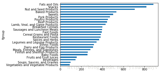
import matplotlib.pyplot as plt
result=ndata.groupby(['nutrient','fgroup'])['value'].quantile(0.5)
result['Energy'].sort_values().plot(kind='barh')
plt.show()
by_nutrient=ndata.groupby(['nutgroup','nutrient'])
get_maximum=lambda x:x.xs(x.value.idxmax())
get_miximum=lambda x:x.xs(x.value.idxmix())
max_foods=by_nutrient.apply(get_maximum)[['value','food']]
max_foods.food=max_foods.food.str[:50]
max_foods.ix['Amino Acids']['food']
nutrient
Alanine                           Gelatins, dry powder, unsweetened
Arginine                               Seeds, sesame flour, low-fat
Aspartic acid                                   Soy protein isolate
Cystine                Seeds, cottonseed flour, low fat (glandless)
Glutamic acid                                   Soy protein isolate
Glycine                           Gelatins, dry powder, unsweetened
Histidine                Whale, beluga, meat, dried (Alaska Native)
Hydroxyproline    KENTUCKY FRIED CHICKEN, Fried Chicken, ORIGINA...
Isoleucine        Soy protein isolate, PROTEIN TECHNOLOGIES INTE...
Leucine           Soy protein isolate, PROTEIN TECHNOLOGIES INTE...
Lysine            Seal, bearded (Oogruk), meat, dried (Alaska Na...
Methionine                    Fish, cod, Atlantic, dried and salted
Phenylalanine     Soy protein isolate, PROTEIN TECHNOLOGIES INTE...
Proline                           Gelatins, dry powder, unsweetened
Serine            Soy protein isolate, PROTEIN TECHNOLOGIES INTE...
Threonine         Soy protein isolate, PROTEIN TECHNOLOGIES INTE...
Tryptophan         Sea lion, Steller, meat with fat (Alaska Native)
Tyrosine          Soy protein isolate, PROTEIN TECHNOLOGIES INTE...
Valine            Soy protein isolate, PROTEIN TECHNOLOGIES INTE...
Name: food, dtype: object