这里主要测试了一下如何对利用caffe的python接口对特征进行可视化,从一次forword中取出param和blob里面的卷积核 和响应的卷积图。我主要是对caffe/models/bvlc_reference_caffenet/路径下的模型和网络配置文件进行了测试,模型为bvlc_reference_caffenet.caffemodel,配置文件为:deploy.prototxt,模型可能需要你自己下载,下载地址为http://dl.caffe.berkeleyvision.org/,当然你也可以用你自己训练得到的模型和网络配置文件,参考代码如下,注意下相应的文件路径:
caffe_visual.py
# -*- coding:utf-8 -*-

import numpy as np
import matplotlib.pyplot as plt
import os
import caffe
import sys
import pickle
import cv2

caffe_root = '/home/rongsong/Downloads/caffe-caffe-0.15/'   # Your caffe diretory path

deployPrototxt = '/home/rongsong/Downloads/caffe-caffe-0.15/models/bvlc_reference_caffenet/deploy.prototxt'
modelFile = '/home/rongsong/Downloads/caffe-caffe-0.15/models/bvlc_reference_caffenet/bvlc_reference_caffenet.caffemodel'
meanFile = 'python/caffe/imagenet/ilsvrc_2012_mean.npy'
#imageListFile = '/home/chenjie/DataSet/CompCars/data/train_test_split/classification/test_model431_label_start0.txt'
#imageBasePath = '/home/chenjie/DataSet/CompCars/data/cropped_image'
#resultFile = 'PredictResult.txt'

#网络初始化
def initilize():
    print 'initilize ... '
    sys.path.insert(0, caffe_root + 'python')
    caffe.set_mode_gpu()
    caffe.set_device(0)
    net = caffe.Net(deployPrototxt, modelFile,caffe.TEST)
    return net

#取出网络中的params和net.blobs的中的数据
def getNetDetails(image, net):
    # input preprocessing: 'data' is the name of the input blob == net.inputs[0]
    transformer = caffe.io.Transformer({'data': net.blobs['data'].data.shape})
    transformer.set_transpose('data', (2,0,1))
    transformer.set_mean('data', np.load(caffe_root + meanFile ).mean(1).mean(1)) # mean pixel
    transformer.set_raw_scale('data', 255)
    # the reference model operates on images in [0,255] range instead of [0,1]
    transformer.set_channel_swap('data', (2,1,0))
    # the reference model has channels in BGR order instead of RGB
    # set net to batch size of 50
    net.blobs['data'].reshape(1,3,227,227)

    net.blobs['data'].data[...] = transformer.preprocess('data', caffe.io.load_image(image))
    out = net.forward()

    #网络提取conv1的卷积核
    filters = net.params['conv1'][0].data
    with open('FirstLayerFilter.pickle','wb') as f:
       pickle.dump(filters,f)
    vis_square(filters.transpose(0, 2, 3, 1))
    #conv1的特征图
    feat = net.blobs['conv1'].data[0, :36]
    with open('FirstLayerOutput.pickle','wb') as f:
       pickle.dump(feat,f)
    vis_square(feat,padval=1)
    pool = net.blobs['pool1'].data[0,:36]
    with open('pool1.pickle','wb') as f:
       pickle.dump(pool,f)
    vis_square(pool,padval=1)


# 此处将卷积图和进行显示,
def vis_square(data, padsize=1, padval=0 ):
    data -= data.min()
    data /= data.max()

    #让合成图为方
    n = int(np.ceil(np.sqrt(data.shape[0])))
    padding = ((0, n ** 2 - data.shape[0]), (0, padsize), (0, padsize)) + ((0, 0),) * (data.ndim - 3)
    data = np.pad(data, padding, mode='constant', constant_values=(padval, padval))
    #合并卷积图到一个图像中

    data = data.reshape((n, n) + data.shape[1:]).transpose((0, 2, 1, 3) + tuple(range(4, data.ndim + 1)))
    data = data.reshape((n * data.shape[1], n * data.shape[3]) + data.shape[4:])
    print data.shape
    plt.imshow(data)
    plt.show()

if __name__ == "__main__":
   net = initilize()
   testimage = '/home/rongsong/Pictures/car0.jpg'     # Your test picture path
   getNetDetails(testimage, net)
测试图片及结果如下:
(a)输入的测试图像

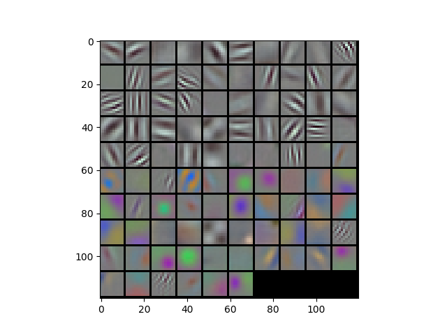
(b)第一层的卷积核和卷积图,可以看到一些明显的边缘轮廓,左侧是相应的卷积核

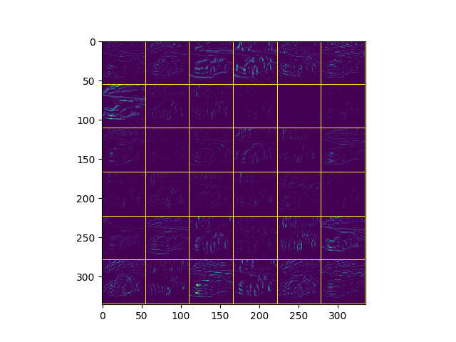
(c)第一个Pooling层的特征图
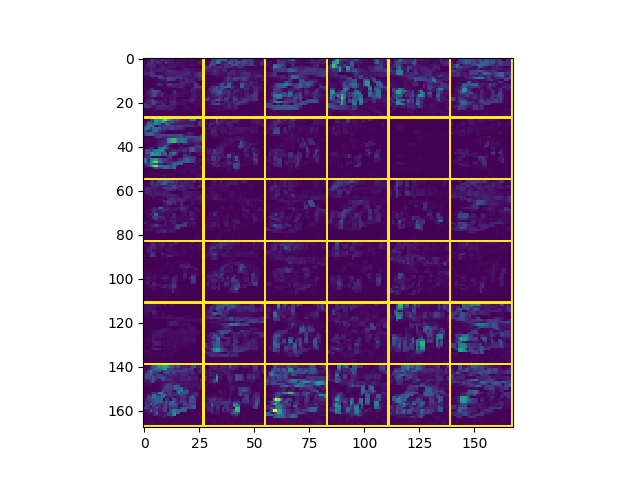
(d)第二层卷积特征图
参考链接:https://www.cnblogs.com/louyihang-loves-baiyan/p/5134671.html