MINIST 手写数字识别数据集,由Yann LeCun所收集,CNN创始人
train:60000
test:10000
本文用Multilayer Perceptron(MLP)的方法,来进行MINIST的识别
1 下载MNIST数据集
1.1 导入Keras及相关模块
import numpy as np
import pandas as pd
from keras.utils import np_utils
np.random.seed(10)
Output
Using TensorFlow backend.
Keras自动以TensorFlow作为Backend
from keras.datasets import mnist #导入MNIST模块1.2 读取MINIST数据集
没有的话会自动下载
(x_train_image, y_train_label), (x_test_image, y_test_label) = mnist.load_data()output
Downloading data from https://s3.amazonaws.com/img-datasets/mnist.npz
11493376/11490434 [==============================] - 7s 1us/step
1.3 查看MNIST数据
输入指令查看已下载的数据集
ll ~/.keras/datasets/mnist.npz
print(np.shape(x_train_image))
print(np.shape(y_train_label))
print(np.shape(x_test_image))
print(np.shape(y_test_label))
output
(60000, 28, 28)
(60000,)
(10000, 28, 28)
(10000,)
3维如下
2 显示data
2.1 显示单个training images and label
import matplotlib.pyplot as plt
def plot_image(image):
    fig = plt.gcf()
    fig.set_size_inches(2, 2) # 设置图片大小
    plt.imshow(image, cmap='binary') #显示灰度图
    plt.savefig('5.png')
    plt.show()
plot_image(x_train_image[0])
y_train_label[0]
Output
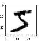
5
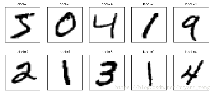
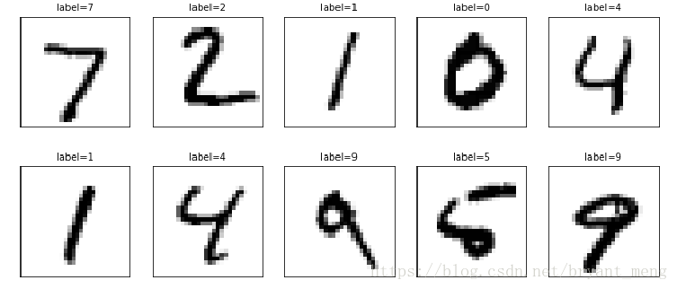
2.2 显示多项training images and label
def plot_images_labels_prediction(images,labels,prediction,idx,num=10):
    '''
    prediction:预测结果
    idx:开始显示的数据的index
    num:要显示的数据项数
    '''
    fig = plt.gcf()
    fig.set_size_inches(12, 14)
    if num>25: num=25 # 显示图片的数量不超过25
    for i in range(0, num):
        ax=plt.subplot(5,5, 1+i) # 建立subgraph
        ax.imshow(images[idx], cmap='binary') # 画出subgraph
        title= "label=" +str(labels[idx]) #设置subgraph title
        if len(prediction)>0: #如果传入了预测结果
            title+=",predict="+str(prediction[idx])
        ax.set_title(title,fontsize=10)  # 设置子图的标题
        ax.set_xticks([]);ax.set_yticks([])   #不显示x轴和y轴坐标
        idx+=1 # 读取下一张图片
    plt.show()
调用
plot_images_labels_prediction(x_train_image,y_train_label,[],0,10)Output
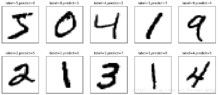
随便加个预测结果
Prediction = []
for i in range(0,10):
    Prediction.append(i)
plot_images_labels_prediction(x_train_image,y_train_label,Prediction,0,10)
Output
看看测试集的
plot_images_labels_prediction(x_test_image,y_test_label,[],0,10)Output
3 Image pre-processing
3.1 把图片变成向量并转化为Float
28×28的图片,转化为1×784向量
x_Train =x_train_image.reshape(60000, 784).astype('float32')
x_Test = x_test_image.reshape(10000, 784).astype('float32')
print ('x_train:',x_Train.shape)
print ('x_test:',x_Test.shape)
Output
x_train: (60000, 784)
x_test: (10000, 784)
3.2 把图片的数字标准化(normalize)
像素值0-255,最简单的方式就是除以255
x_Train_normalize = x_Train/ 255
x_Test_normalize = x_Test/ 255type(x_Train_normalize)Output
numpy.ndarray
操作以后,所有的数字都介于0-1之间
4 Label pre-processing
One-Hot Encoding
y_train_label[:3]Output
array([5, 0, 4], dtype=uint8)
调用keras
y_TrainOneHot = np_utils.to_categorical(y_train_label)
y_TestOneHot = np_utils.to_categorical(y_test_label)y_TrainOneHot[:3]Output
array([[0., 0., 0., 0., 0., 1., 0., 0., 0., 0.],
       [1., 0., 0., 0., 0., 0., 0., 0., 0., 0.],
       [0., 0., 0., 0., 1., 0., 0., 0., 0., 0.]], dtype=float32)
5 Multilayer Perceptron 256
model = Sequential()
model.add
model.compile
model.fit
model.evaluate
model.predict
5.1 Build Model
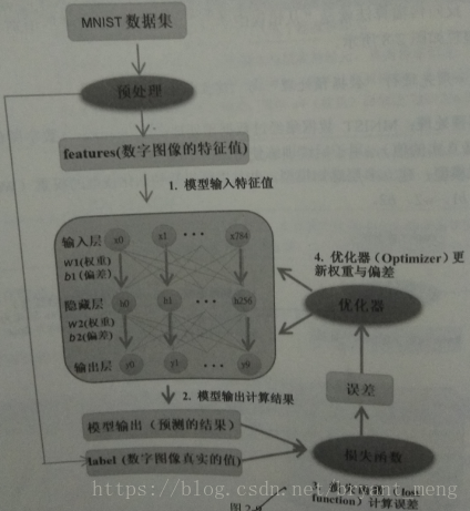
- input layer:784
- hidden layer:256
- output layer:10
from keras.models import Sequential
from keras.layers import Dense

 #蛋糕架子,后续的组件用model.add的方法
model = Sequential()

# 建立输入层和隐藏层
model.add(Dense(units=256, #隐藏层神经元个数256
                input_dim=784, #输入层784
                kernel_initializer='normal',#正态分布的随机数来初始化weight and bias
                activation='relu')) # activation function is relu
# 建立输出层
model.add(Dense(units=10, #输出层的神经元个数为10个
                kernel_initializer='normal', #正态分布的随机数来初始化weight and bias
                activation='softmax'))# 激活函数为softmax,其可将输出转化为预测的概率
Note: 第二个Dense不需要设置input_dim,Keras会自动按照上一层的units是256个神经元,设置这一层的input_dim为256个神经元
5.2 查看模型摘要
print(model.summary())Output
_________________________________________________________________
Layer (type)                 Output Shape              Param #
=================================================================
dense_1 (Dense)              (None, 256)               200960
_________________________________________________________________
dense_2 (Dense)              (None, 10)                2570
=================================================================
Total params: 203,530
Trainable params: 203,530
Non-trainable params: 0
_________________________________________________________________
None
training parameters 计算方法:
784*256+256 = 200960
256*10+10 = 2570
200960+2570 = 203530
参数越多,模型越复杂
5.3 Training process
model.compile(loss='categorical_crossentropy',optimizer='adam', metrics=['accuracy'])- loss:cross entropy
- optimizer:adam 加速收敛
- metrics :设置模型评估的方式是准确率
train_history =model.fit(x=x_Train_normalize,
                         y=y_Train_OneHot,validation_split=0.2,
epochs=10, batch_size=200,verbose=2)- validation_split = 0.2: training data 和 validation data 比例8:2,60000*80% = 48000
- epochs=10:训练集(48000)跑10次
- batch_size=200,200个图片一次step,跑完一个epoch,48000÷200 = 240 steps
- verbose=2:显示训练过程
Output
Train on 48000 samples, validate on 12000 samples
Epoch 1/10
- 4s - loss: 0.4434 - acc: 0.8813 - val_loss: 0.2193 - val_acc: 0.9400
Epoch 2/10
- 1s - loss: 0.1916 - acc: 0.9451 - val_loss: 0.1557 - val_acc: 0.9556
Epoch 3/10
- 1s - loss: 0.1358 - acc: 0.9616 - val_loss: 0.1262 - val_acc: 0.9643
Epoch 4/10
- 1s - loss: 0.1030 - acc: 0.9704 - val_loss: 0.1126 - val_acc: 0.9677
Epoch 5/10
- 1s - loss: 0.0813 - acc: 0.9774 - val_loss: 0.0988 - val_acc: 0.9718
Epoch 6/10
- 1s - loss: 0.0661 - acc: 0.9816 - val_loss: 0.0941 - val_acc: 0.9719
Epoch 7/10
- 1s - loss: 0.0545 - acc: 0.9850 - val_loss: 0.0916 - val_acc: 0.9735
Epoch 8/10
- 1s - loss: 0.0457 - acc: 0.9878 - val_loss: 0.0834 - val_acc: 0.9763
Epoch 9/10
- 1s - loss: 0.0380 - acc: 0.9903 - val_loss: 0.0822 - val_acc: 0.9761
Epoch 10/10
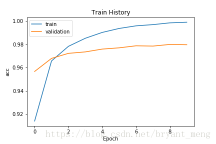
- 1s - loss: 0.0316 - acc: 0.9917 - val_loss: 0.0799 - val_acc: 0.97685.4 可视化训练过程
import matplotlib.pyplot as plt
def show_train_history(train_history,train,validation):
    plt.plot(train_history.history[train])
    plt.plot(train_history.history[validation])
    plt.title('Train History')
    plt.ylabel(train)
    plt.xlabel('Epoch')
    plt.legend(['train', 'validation'], loc='upper left')
    plt.savefig('1.png')
    plt.show()
调用
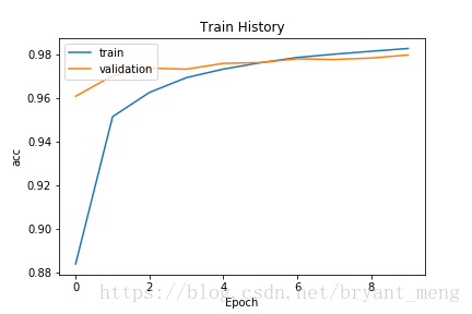
show_train_history(train_history,'acc','val_acc')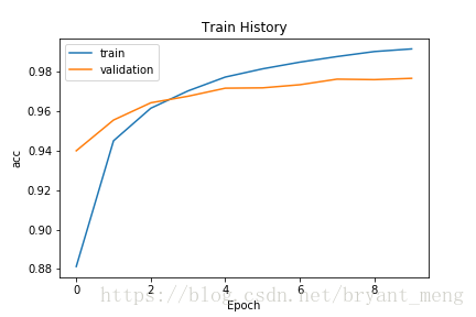
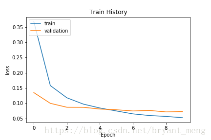
show_train_history(train_history,'loss','val_loss')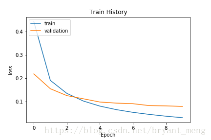
Q:为何训练集的accuracy 比 验证机的 accuracy要高
以训练的数据来计算准确率,因为相同的数据已经训练过了,又拿来计算准确率,所以准确率会比较高(做过的卷子再拿来测试)
5.5 评估准确率
scores = model.evaluate(x_Test_normalize, y_Test_OneHot)
print()
print('accuracy=',scores[1])
Output
10000/10000 [==============================] - 1s 61us/step

accuracy= 0.9764
5.6 进行预测
prediction=model.predict_classes(x_Test)# x_Test 是读入的测试集
prediction
Output
array([7, 2, 1, ..., 4, 5, 6])用之前的plot_images_labels_prediction 函数可视化一下一些例子
import matplotlib.pyplot as plt
def plot_images_labels_prediction(images,labels,prediction,
                                  idx,num=10):
    fig = plt.gcf()
    fig.set_size_inches(12, 14)
    if num>25: num=25
    for i in range(0, num):
        ax=plt.subplot(5,5, 1+i)
        ax.imshow(images[idx], cmap='binary')
        title= "label=" +str(labels[idx])
        if len(prediction)>0:
            title+=",predict="+str(prediction[idx])
        ax.set_title(title,fontsize=10)
        ax.set_xticks([]);ax.set_yticks([])
        idx+=1
    plt.savefig('1.png')
    plt.show()
调用,显示340-349编号图片
Output
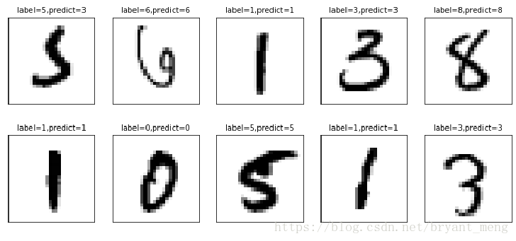
发现有一张错了,5识别成了3,不过看上去挺像的
5.7 Confusion Matrix
import pandas as pd
pd.crosstab(y_test_label,prediction,
rownames=['label'],colnames=['predict'])- 行:测试集的label
- 列:模型的预测值
Output
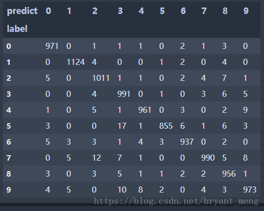
对角线是预测正确的数量
5.8 建立真实值与预测值的Data Frame
df = pd.DataFrame({'label':y_test_label, 'predict':prediction})
# 类型 pandas.core.frame.DataFrame
# 长度为10000
print(df[:5]) #显示前5项
Output
   label  predict
0      7        7
1      2        2
2      1        1
3      0        0
4      4        4
Note:不打印的画,会自动画成如confusion matrix 的表格
查看真实值是5,预测成3的数据
a = df[(df.label==5)&(df.predict==3)]
print(a)
len(a)
Outout
      label  predict
340       5        3
1003      5        3
1393      5        3
2035      5        3
2526      5        3
2597      5        3
2810      5        3
3117      5        3
3902      5        3
4271      5        3
4355      5        3
4360      5        3
5937      5        3
5972      5        3
6028      5        3
6043      5        3
6598      5        3
17
第一列的是图片编号,0开始
6 Multilayer Perceptron 1000
- input layer:784
- hidden layer:1000
- output layer:10
6.1 Data processing and Build Model
# 预处理
from keras.utils import np_utils
import numpy as np
np.random.seed(10)
from keras.datasets import mnist
(x_train_image,y_train_label),\
(x_test_image,y_test_label)= mnist.load_data()
x_Train =x_train_image.reshape(60000, 784).astype('float32')
x_Test = x_test_image.reshape(10000, 784).astype('float32')
x_Train_normalize = x_Train / 255
x_Test_normalize = x_Test / 255
y_Train_OneHot = np_utils.to_categorical(y_train_label)
y_Test_OneHot = np_utils.to_categorical(y_test_label)
# 建立模型
from keras.models import Sequential
from keras.layers import Dense
model = Sequential()
model.add(Dense(units=1000,
                input_dim=784,
                kernel_initializer='normal',
                activation='relu'))
model.add(Dense(units=10,
                kernel_initializer='normal',
                activation='softmax'))
6.2 查看模型
print(model.summary())Output
_________________________________________________________________
Layer (type)                 Output Shape              Param #
=================================================================
dense_1 (Dense)              (None, 1000)              785000
_________________________________________________________________
dense_2 (Dense)              (None, 10)                10010
=================================================================
Total params: 795,010
Trainable params: 795,010
Non-trainable params: 0
_________________________________________________________________
None
6.3 Training
model.compile(loss='categorical_crossentropy',
              optimizer='adam', metrics=['accuracy'])
train_history=model.fit(x=x_Train_normalize,
                        y=y_Train_OneHot,validation_split=0.2,
                        epochs=10, batch_size=200,verbose=2)
Output
Train on 48000 samples, validate on 12000 samples
Epoch 1/10
 - 9s - loss: 0.2983 - acc: 0.9141 - val_loss: 0.1525 - val_acc: 0.9568
Epoch 2/10
 - 4s - loss: 0.1181 - acc: 0.9658 - val_loss: 0.1079 - val_acc: 0.9680
Epoch 3/10
 - 4s - loss: 0.0759 - acc: 0.9784 - val_loss: 0.0928 - val_acc: 0.9723
Epoch 4/10
 - 4s - loss: 0.0516 - acc: 0.9853 - val_loss: 0.0883 - val_acc: 0.9736
Epoch 5/10
 - 4s - loss: 0.0358 - acc: 0.9903 - val_loss: 0.0749 - val_acc: 0.9760
Epoch 6/10
 - 4s - loss: 0.0254 - acc: 0.9938 - val_loss: 0.0750 - val_acc: 0.9771
Epoch 7/10
 - 4s - loss: 0.0182 - acc: 0.9960 - val_loss: 0.0737 - val_acc: 0.9788
Epoch 8/10
 - 4s - loss: 0.0134 - acc: 0.9970 - val_loss: 0.0735 - val_acc: 0.9786
Epoch 9/10
 - 4s - loss: 0.0090 - acc: 0.9986 - val_loss: 0.0708 - val_acc: 0.9800
Epoch 10/10
 - 4s - loss: 0.0063 - acc: 0.9991 - val_loss: 0.0718 - val_acc: 0.9798
6.4 可视化训练过程
用前面的show_train_history函数
看精度
show_train_history(train_history,'acc','val_acc')Output
看损失
show_train_history(train_history,'loss','val_loss')Output
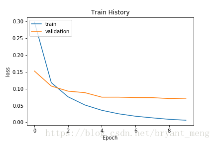
可以看出,在训练集的表现比验证集好多了,比刚才的模型更过拟合
6.5 评估模型
scores = model.evaluate(x_Test_normalize, y_Test_OneHot)
print()
print('accuracy=',scores[1])
Output
10000/10000 [==============================] - 2s 156us/step

accuracy= 0.9796
7 Multilayer Perceptron 加 DropOut
减缓下过拟合的问题
7.1 Build Model
from keras.models import Sequential
from keras.layers import Dense
from keras.layers import Dropout
model = Sequential()
model.add(Dense(units=1000,
                input_dim=784,
                kernel_initializer='normal',
                activation='relu'))
model.add(Dropout(0.5))# 新增
model.add(Dense(units=10,
                kernel_initializer='normal',
                activation='softmax'))
print(model.summary())
Output
Layer (type)                 Output Shape              Param #
=================================================================
dense_1 (Dense)              (None, 1000)              785000
_________________________________________________________________
dropout_1 (Dropout)          (None, 1000)              0
_________________________________________________________________
dense_2 (Dense)              (None, 10)                10010
=================================================================
Total params: 795,010
Trainable params: 795,010
Non-trainable params: 0
_________________________________________________________________
None
7.2 Training process
model.compile(loss='categorical_crossentropy',
              optimizer='adam', metrics=['accuracy'])
train_history=model.fit(x=x_Train_normalize,
                        y=y_Train_OneHot,validation_split=0.2,
                        epochs=10, batch_size=200,verbose=2)
Output
Train on 48000 samples, validate on 12000 samples
Epoch 1/10
 - 8s - loss: 0.3560 - acc: 0.8930 - val_loss: 0.1703 - val_acc: 0.9528
Epoch 2/10
 - 4s - loss: 0.1596 - acc: 0.9526 - val_loss: 0.1190 - val_acc: 0.9667
Epoch 3/10
 - 4s - loss: 0.1158 - acc: 0.9664 - val_loss: 0.1002 - val_acc: 0.9713
Epoch 4/10
 - 4s - loss: 0.0917 - acc: 0.9733 - val_loss: 0.0857 - val_acc: 0.9744
Epoch 5/10
 - 4s - loss: 0.0741 - acc: 0.9775 - val_loss: 0.0766 - val_acc: 0.9774
Epoch 6/10
 - 4s - loss: 0.0629 - acc: 0.9805 - val_loss: 0.0745 - val_acc: 0.9769
Epoch 7/10
 - 4s - loss: 0.0534 - acc: 0.9838 - val_loss: 0.0708 - val_acc: 0.9779
Epoch 8/10
 - 4s - loss: 0.0465 - acc: 0.9853 - val_loss: 0.0703 - val_acc: 0.9781
Epoch 9/10
 - 4s - loss: 0.0420 - acc: 0.9871 - val_loss: 0.0697 - val_acc: 0.9793
Epoch 10/10
 - 4s - loss: 0.0367 - acc: 0.9888 - val_loss: 0.0651 - val_acc: 0.9800
训练和验证表现差不多,减缓了过拟合
7.3 评估模型
scores = model.evaluate(x_Test_normalize, y_Test_OneHot)
print()
print('accuracy=',scores[1])
Output
10000/10000 [==============================] - 2s 153us/step

accuracy= 0.9795
8 Multilayer Perceptron two hidden layer
8.1 Build Model
from keras.models import Sequential
from keras.layers import Dense
from keras.layers import Dropout
model = Sequential()

model.add(Dense(units=1000,
                input_dim=784,
                kernel_initializer='normal',
                activation='relu'))
model.add(Dropout(0.5))

model.add(Dense(units=1000,
                kernel_initializer='normal',
                activation='relu'))
model.add(Dropout(0.5))

model.add(Dense(units=10,
                kernel_initializer='normal',
                activation='softmax'))

print(model.summary())
Output
_________________________________________________________________
Layer (type)                 Output Shape              Param #
=================================================================
dense_1 (Dense)              (None, 1000)              785000
_________________________________________________________________
dropout_1 (Dropout)          (None, 1000)              0
_________________________________________________________________
dense_2 (Dense)              (None, 1000)              1001000
_________________________________________________________________
dropout_2 (Dropout)          (None, 1000)              0
_________________________________________________________________
dense_3 (Dense)              (None, 10)                10010
=================================================================
Total params: 1,796,010
Trainable params: 1,796,010
Non-trainable params: 0
_________________________________________________________________
None
8.2 Training process
model.compile(loss='categorical_crossentropy',
              optimizer='adam', metrics=['accuracy'])
train_history=model.fit(x=x_Train_normalize,
                        y=y_Train_OneHot,validation_split=0.2,
                        epochs=10, batch_size=200,verbose=2)
Output
Train on 48000 samples, validate on 12000 samples
Epoch 1/10
 - 13s - loss: 0.3679 - acc: 0.8842 - val_loss: 0.1349 - val_acc: 0.9610
Epoch 2/10
 - 6s - loss: 0.1579 - acc: 0.9516 - val_loss: 0.0997 - val_acc: 0.9704
Epoch 3/10
 - 6s - loss: 0.1179 - acc: 0.9628 - val_loss: 0.0868 - val_acc: 0.9738
Epoch 4/10
 - 6s - loss: 0.0971 - acc: 0.9695 - val_loss: 0.0867 - val_acc: 0.9734
Epoch 5/10
 - 6s - loss: 0.0843 - acc: 0.9734 - val_loss: 0.0809 - val_acc: 0.9761
Epoch 6/10
 - 6s - loss: 0.0746 - acc: 0.9764 - val_loss: 0.0785 - val_acc: 0.9764
Epoch 7/10
 - 6s - loss: 0.0650 - acc: 0.9788 - val_loss: 0.0746 - val_acc: 0.9782
Epoch 8/10
 - 6s - loss: 0.0597 - acc: 0.9803 - val_loss: 0.0763 - val_acc: 0.9778
Epoch 9/10
 - 5s - loss: 0.0567 - acc: 0.9816 - val_loss: 0.0716 - val_acc: 0.9785
Epoch 10/10
 - 5s - loss: 0.0525 - acc: 0.9829 - val_loss: 0.0724 - val_acc: 0.9799
8.3 可视化一下训练过程
8.4 评估模型
scores = model.evaluate(x_Test_normalize, y_Test_OneHot)
print()
print('accuracy=',scores[1])
Output
10000/10000 [==============================] - 2s 161us/step

accuracy= 0.9807
总结:MLP有上限,准确率98%左右
声明
声明:代码源于《TensorFlow+Keras深度学习人工智能实践应用》 林大贵版,引用、转载请注明出处,谢谢,如果对书本感兴趣,买一本看看吧!!!