目录
4.mRMR(minimum Redundancy Maximum Relevance)
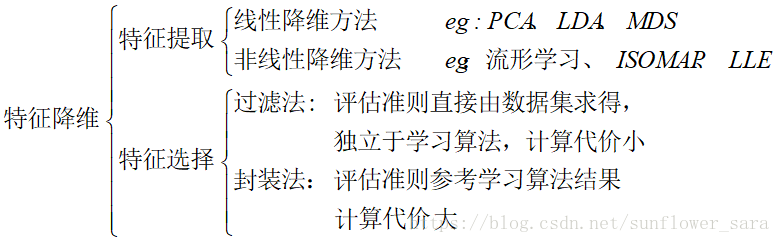
一、数据降维
1.特征提取
将原有特征窄间进行某种形式的变换,以得到新的特征。
特征的理解性很差。
2.特征选择
从原特征集中选择一个最优特征子集,保留了原有特征集的大部分类别信息。
剔除无关的或者冗余的特征,更精确的模型,更容易理解。
分类如下:
二、特征选择方法
1.F_score
计算公式如下:
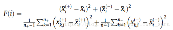

特点:
衡量两类特征之间的间距
F值越大,此特征的辨别力越强
参考文献:
Polat K, Güneş S. A new feature selection method on classification of medical datasets: Kernel F-score feature selection[J]. Expert Systems with Applications, 2009, 36(7):10367-10373.
2.relief,reliefF
区别:
relief为二分类的度量,reliefF为推广到多分类的度量
reliefF公式如下:
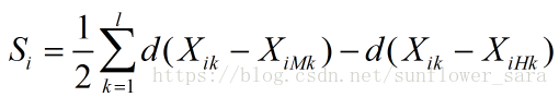
算法流程:
算法从训练集D中随机选择一个样本R,然后从和R同类的样本中寻找最近邻样本H,称为Near Hit,从和R不同类的样本中寻找最近邻样本M,称为NearMiss,然后根据以下规则更新每个特征的权重:如果R和Near Hit在某个特征上的距离小于R和Near Miss上的距离,则说明该特征对区分同类和不同类的最近邻是有益的,则增加该特征的权重;反之,如果R和Near Hit在某个特征的距离大于R和Near Miss上的距离,说明该特征对区分同类和不同类的最近邻起负面作用,则降低该特征的权重。以上过程重复m次,最后得到各特征的平均权重。特征的权重越大,表示该特征的分类能力越强,反之,表示该特征分类能力越弱。Relief算法的运行时间随着样本的抽样次数m和原始特征个数N的增加线性增加,因而运行效率非常高。但是算法会赋予所有和类别相关性高的特征较高的权重,所以算法的局限性在于不能有效的去除冗余特征。
概括一下流程:
随机选择一个样本R
从和R同类的样本中寻找最近邻样本H;从和R不同类的样本中寻找最近邻样本M
根据特征与临近样本的距离进行权重更新
以上过程重复m次,最后得到各特征的平均权重。
优点:运行效率高
缺点:只赋予所有和类别相关性高的特征较高的权重,不能有效的去除冗余特征。
参考文献:
J. Tang, S. Alelyani, and H. Liu, Feature selection for classification: a review, Data Classification: Algorithms and Applications, 37: 2014.
3.Fisher
参考文献:
编辑:Charu C. Aggarwal, IBM T. J. Watson Research Center, Yorktown Heights, New York, USA
书名:Data classification (后面的名字记不清了)
function [W,index,Data_Fisher_sort] = fsFisher(Data,Label)
%Fisher Score, use the N var formulation
%   X, the data, each raw is an instance
%   Y, the label in 1 2 3 ... format

numClass = max(Label);
[numData, numFeature] = size(Data);
out.W = zeros(1,numFeature);

% statistic for classes
cIDX = cell(numClass,1);
n_i = zeros(numClass,1);
for j = 1:numClass
    cIDX{j} = find(Label(:)==j);
    n_i(j) = length(cIDX{j});
end

% calculate score for each features
for i = 1:numFeature
    temp1 = 0;
    temp2 = 0;
    f_i = Data(:,i);
    u_i = mean(f_i);

    for j = 1:numClass
        u_cj = mean(f_i(cIDX{j}));
        var_cj = var(f_i(cIDX{j}),1);
        temp1 = temp1 + n_i(j) * (u_cj-u_i)^2;
        temp2 = temp2 + n_i(j) * var_cj;
    end

    if temp1 == 0
        out.W(i) = 0;
    else
        if temp2 == 0
            out.W(i) = 100;
        else
            out.W(i) = temp1/temp2;
        end
    end
end

[~, out.fList] = sort(out.W, 'descend');
out.prf = 1;

W=out.W;
index=(out.fList)';

Data_relieF_sort=zeros(numData,numFeature);
for i=1:numFeature
    Data_Fisher_sort(1:numData,i)= Data(1:numData,index(i));
end


end
4.LaplacianScore
参考文献:
编辑:Charu C. Aggarwal, IBM T. J. Watson Research Center, Yorktown Heights, New York, USA
书名:Data classification (后面的名字记不清了)
function [Y,flip_index,Data_Laplacian_sort] = LaplacianScore(Data, W)
%	Usage:
%	[Y] = LaplacianScore(X, W)
%
%	X: Rows of vectors of data points    Data
%	W: The affinity matrix.
%	Y: Vector of (1-LaplacianScore) for each feature.
%      The features with larger y are more important.
%
%    Examples:
%
%       fea = rand(50,70);
%       options = [];
%       options.Metric = 'Cosine';
%       options.NeighborMode = 'KNN';
%       options.k = 5;
%       options.WeightMode = 'Cosine';
%       W = constructW(fea,options);
%
%       LaplacianScore = LaplacianScore(fea,W);
%       [junk, index] = sort(-LaplacianScore);
%
%       newfea = fea(:,index);
%       %the features in newfea will be sorted based on their importance.
%
%	Type "LaplacianScore" for a self-demo.
%
% See also constructW
%
%Reference:
%
%   Xiaofei He, Deng Cai and Partha Niyogi, "Laplacian Score for Feature Selection".
%   Advances in Neural Information Processing Systems 18 (NIPS 2005),
%   Vancouver, Canada, 2005.
%
%   Deng Cai, 2004/08


if nargin == 0, selfdemo; return; end

[nSmp,nFea] = size(Data);

if size(W,1) ~= nSmp
    error('W is error');
end

D = full(sum(W,2));
L = W;

allone = ones(nSmp,1);


tmp1 = D'*Data;

D = sparse(1:nSmp,1:nSmp,D,nSmp,nSmp);

DPrime = sum((Data'*D)'.*Data)-tmp1.*tmp1/sum(diag(D));
LPrime = sum((Data'*L)'.*Data)-tmp1.*tmp1/sum(diag(D));

DPrime(find(DPrime < 1e-12)) = 10000;

Y = LPrime./DPrime;
Y = Y';
Y = full(Y);


[junk, flip_index] = sort(Y,'descend');

Data_Laplacian_sort=zeros(nSmp,nFea);
for i=1:nFea
    Data_Laplacian_sort(1:nSmp,i)= Data(1:nSmp,flip_index(i));
end


% %---------------------------------------------------
% function selfdemo
% % ====== Self demo using IRIS dataset
% % ====== 1. Plot IRIS data after LDA for dimension reduction to 2D
% load iris.dat
%
% feaNorm = mynorm(iris(:,1:4),2);
% fea = iris(:,1:4) ./ repmat(max(1e-10,feaNorm),1,4);
%
% options = [];
% options.Metric = 'Cosine';
% options.NeighborMode = 'KNN';
% options.WeightMode = 'Cosine';
% options.k = 3;
%
% W = constructW(fea,options);
%
% [LaplacianScore] = feval(mfilename,iris(:,1:4),W);
% [junk, index] = sort(-LaplacianScore);
%
% index1 = find(iris(:,5)==1);
% index2 = find(iris(:,5)==2);
% index3 = find(iris(:,5)==3);
% figure;
% plot(iris(index1, index(1)), iris(index1, index(2)), '*', ...
%      iris(index2, index(1)), iris(index2, index(2)), 'o', ...
%      iris(index3, index(1)), iris(index3, index(2)), 'x');
% legend('Class 1', 'Class 2', 'Class 3');
% title('IRIS data onto the first and second feature (Laplacian Score)');
% axis equal; axis tight;
%
% figure;
% plot(iris(index1, index(3)), iris(index1, index(4)), '*', ...
%      iris(index2, index(3)), iris(index2, index(4)), 'o', ...
%      iris(index3, index(3)), iris(index3, index(4)), 'x');
% legend('Class 1', 'Class 2', 'Class 3');
% title('IRIS data onto the third and fourth feature (Laplacian Score)');
% axis equal; axis tight;
%
% disp('Laplacian Score:');
% for i = 1:length(LaplacianScore)
%     disp(num2str(LaplacianScore(i)));
% end
4.mRMR(minimum Redundancy Maximum Relevance)
最大相关最小冗余
特征对类别相关度度量:
Max:

使用各个特征与类别的信息增益的均值
特征之间冗余度度量:
Min:
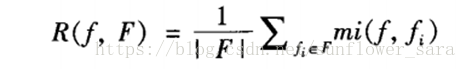
使用特征和特征之间的互信息加和再除以子集中特征个数的平方
最终标准: max Φ(D,R), Φ=D−R

相关程序包 http://penglab.janelia.org/proj/mRMR/
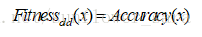
5.GA
遗传算法通过交叉、选择、变异等,对染色体进行变化
通过libsvm对染色体筛选出的特征进行评判,得到accuracy
不断优化适应度函数为最大
6.GA_mRMR
新的适应度函数:
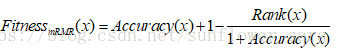
rank是根据mRMR的排序值
7.基于稀疏表示的特征筛选SRC
意欲用尽可能少的非0系数表示信号的主要信息,从而简化信号处理问题的求解过程
比如有110例数据,每个数据有197维的特征
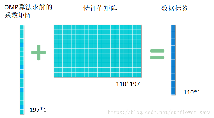
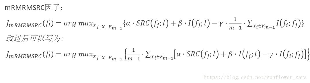
8.mRMRMSRC
先给一下互信息的公式:
I(X,Y)=∫X∫YP(X,Y)logP(X,Y)P(X)P(Y)、
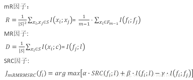
参考文献:
Tongtong Liu et al. A mRMRMSRC feature selection method for radiomics approach. 2017 39th Annual International Conference of the IEEE Engineering in Medicine and Biology Society (EMBC), Jeju Island, South Korea, 2017:616-619.
先给一下互信息的公式:
I(X,Y)=∫X∫YP(X,Y)logP(X,Y)P(X)P(Y)