正则化
- 过拟合:神经网络模型在训练数据集上的准确率较高,在新的数据进行预测或分类时准确率较低,说明模型的泛化能力差。
- 正则化:在损失函数中给每个参数 w 加上权重,引入模型复杂度指标,从而抑制模型噪声,减小过拟合。
- 使用正则化后,损失函数 loss 变为两项之和:
loss = loss(y 与 y_) + REGULARIZER*loss(w)
其中,第一项是预测结果与标准答案之间的差距,如交叉熵、均方误差等;第二项是正则化计算结果。 正则化计算方法:
L1正则化:
- 计算公式:
- 用 Tesnsorflow 函数表示
RL_1 = tf.contrib.layers.l1_regularizer(REGULARIZER)(w)
- 计算公式:
L2正则化:
- 计算公式:
- 用 Tesnsorflow 函数表示
RL_2 = tf.contrib.layers.l2_regularizer(REGULARIZER)(w)
- 计算公式:
用 Tesnsorflow 函数实现正则化:
tf.add_to_collection('losses', RL_2)
loss = loss_cem + tf.add_n(tf.get_collection('losses'))
示例:
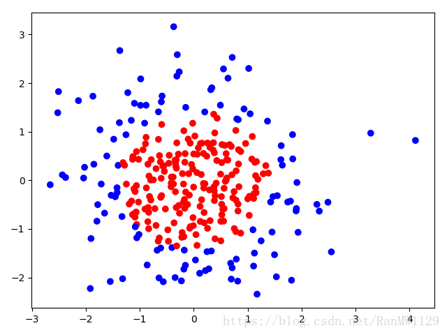
用 300 个符合正态分布的点 作为数据集,根据点 计算生成标注 ,将数据集标注为红色点和蓝色点。
标注规则为:当 时, ,标注为红色;当 时, ,标注为蓝色。
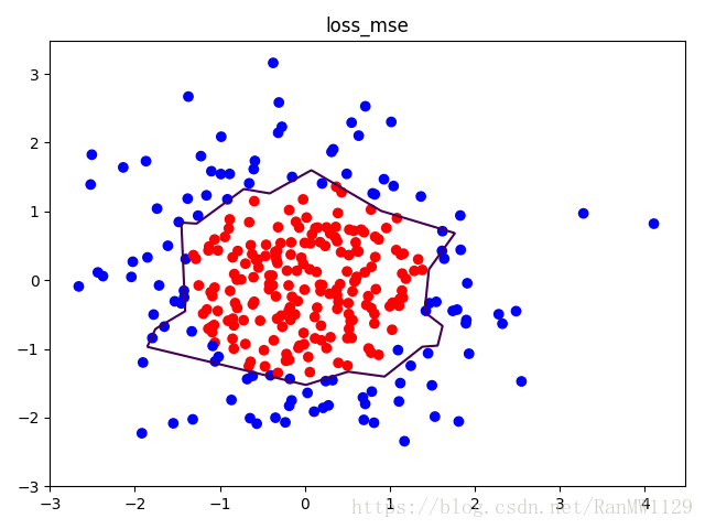
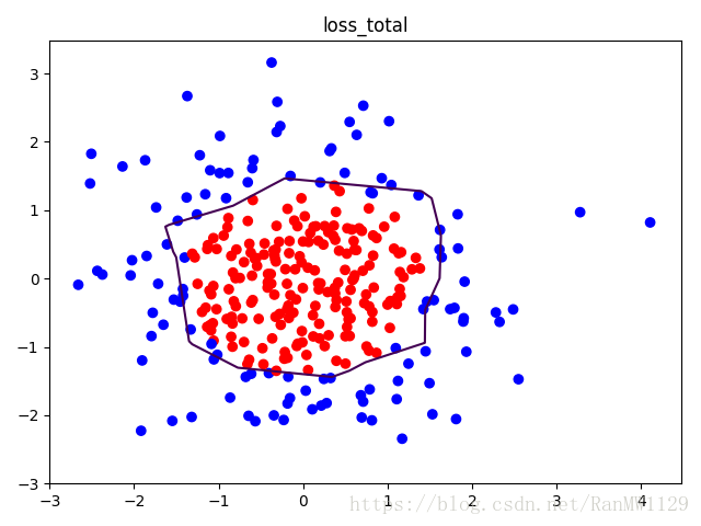
我们分别用无正则化和有正则化两种方法,拟合曲线,把红色点和蓝色点分开。在实际分类时,如果前向传播输出的预测值 接近 1 则为红色点概率越大,接近 0 则为蓝色点概率越大,输出的预测值 为 0.5 是红蓝点概率分界线。import tensorflow as tf import matplotlib.pyplot as plt import numpy as np BATCH_SIZE = 30 SEED = 2 rdm = np.random.RandomState(SEED) X = rdm.randn(300, 2) Y_ = [int(xi[0]*xi[0] + xi[1]*xi[1] < 2) for xi in X] Y_c = [['red' if y else 'blue'] for y in Y_] X = np.vstack(X).reshape(-1, 2) Y_ = np.vstack(Y_).reshape(-1, 1) plt.scatter(X[:,0], X[:,1], c=np.squeeze(Y_c)) plt.show() def get_weight(shape, regularizer): w = tf.Variable(tf.random_normal(shape), dtype=tf.float32) tf.add_to_collection('losses', tf.contrib.layers.l2_regularizer(regularizer)(w)) return w def get_bias(shape): b = tf.Variable(tf.constant(0.01, shape=shape)) return b x = tf.placeholder(tf.float32, shape=(None, 2)) y_ = tf.placeholder(tf.float32, shape=(None, 1)) w1 = get_weight([2, 11], 0.01) b1 = get_bias([11]) y1 = tf.nn.relu(tf.matmul(x, w1) + b1) w2 = get_weight([11, 1], 0.01) b2 = get_bias([1]) y = tf.matmul(y1, w2) + b2 loss_mse = tf.reduce_mean(tf.square(y-y_)) loss_total = loss_mse + tf.add_n(tf.get_collection('losses')) train_step = tf.train.AdamOptimizer(0.0001).minimize(loss_mse) with tf.Session() as sess: sess.run(tf.global_variables_initializer()) STEPS = 40000 for i in range(STEPS): start = (i*BATCH_SIZE) % 300 end = min(start+BATCH_SIZE, 300) sess.run(train_step, feed_dict={x: X[start:end], y_:Y_[start:end]}) if i % 2000 == 0: loss_mse_v = sess.run(loss_mse, feed_dict={x:X, y_:Y_}) print('After %d steps, loss_mse is: %f' % (i, loss_mse_v)) xx, yy = np.mgrid[-3:3:0.01, -3:3:0.01] grid = np.c_[xx.ravel(), yy.ravel()] probs = sess.run(y, feed_dict={x:grid}) probs = probs.reshape(xx.shape) print('w1:', sess.run(w1)) print('b1:', sess.run(b1)) print('w2:', sess.run(w2)) print('b2:', sess.run(b2)) plt.scatter(X[:,0], X[:,1], c=np.squeeze(Y_c)) plt.contour(xx, yy, probs, levels=[.5]) plt.title('loss_mse') plt.show() train_step = tf.train.AdamOptimizer(0.0001).minimize(loss_total) with tf.Session() as sess: sess.run(tf.global_variables_initializer()) STEPS = 40000 for i in range(STEPS): start = (i*BATCH_SIZE) % 300 end = min(start+BATCH_SIZE, 300) sess.run(train_step, feed_dict={x: X[start:end], y_:Y_[start:end]}) if i % 2000 == 0: loss_total_v = sess.run(loss_total, feed_dict={x:X, y_:Y_}) print('After %d steps, loss_total is: %f' % (i, loss_total_v)) xx, yy = np.mgrid[-3:3:0.01, -3:3:0.01] grid = np.c_[xx.ravel(), yy.ravel()] probs = sess.run(y, feed_dict={x:grid}) probs = probs.reshape(xx.shape) print('w1:', sess.run(w1)) print('b1:', sess.run(b1)) print('w2:', sess.run(w2)) print('b2:', sess.run(b2)) plt.scatter(X[:,0], X[:,1], c=np.squeeze(Y_c)) plt.contour(xx, yy, probs, levels=[.5]) plt.title('loss_total') plt.show()可视化数据集:
无正则化:
有正则化:
np.vstack()
def vstack(tup):
    """
    Stack arrays in sequence vertically (row wise).

    This is equivalent to concatenation along the first axis after 1-D arrays
    of shape `(N,)` have been reshaped to `(1,N)`. Rebuilds arrays divided by
    `vsplit`.

    This function makes most sense for arrays with up to 3 dimensions. For
    instance, for pixel-data with a height (first axis), width (second axis),
    and r/g/b channels (third axis). The functions `concatenate`, `stack` and
    `block` provide more general stacking and concatenation operations.

    Parameters
    ----------
    tup : sequence of ndarrays
        The arrays must have the same shape along all but the first axis.
        1-D arrays must have the same length.

    Returns
    -------
    stacked : ndarray
        The array formed by stacking the given arrays, will be at least 2-D.

    See Also
    --------
    stack : Join a sequence of arrays along a new axis.
    hstack : Stack arrays in sequence horizontally (column wise).
    dstack : Stack arrays in sequence depth wise (along third dimension).
    concatenate : Join a sequence of arrays along an existing axis.
    vsplit : Split array into a list of multiple sub-arrays vertically.
    block : Assemble arrays from blocks.

    Examples
    --------
    >>> a = np.array([1, 2, 3])
    >>> b = np.array([2, 3, 4])
    >>> np.vstack((a,b))
    array([[1, 2, 3],
           [2, 3, 4]])

    >>> a = np.array([[1], [2], [3]])
    >>> b = np.array([[2], [3], [4]])
    >>> np.vstack((a,b))
    array([[1],
           [2],
           [3],
           [2],
           [3],
           [4]])

    """
画散点图
plt.scatter (x 坐标, y 坐标, c=”颜色”)收集规定区域内所有的网格坐标点:
xx, yy = np.mgrid[起:止:步长, 起:止:步长] # 找到规定区域以步长为分辨率的行列网格坐标点
grid = np.c_[xx.ravel(), yy.ravel()] # 收集规定区域内所有的网格坐标点
例如:
xx, yy = np.mgrid[0:5, 0:5]
xx
array([[0, 0, 0, 0, 0],
       [1, 1, 1, 1, 1],
       [2, 2, 2, 2, 2],
       [3, 3, 3, 3, 3],
       [4, 4, 4, 4, 4]])
yy
array([[0, 1, 2, 3, 4],
       [0, 1, 2, 3, 4],
       [0, 1, 2, 3, 4],
       [0, 1, 2, 3, 4],
       [0, 1, 2, 3, 4]])
xx.ravel()
array([0, 0, 0, 0, 0, 1, 1, 1, 1, 1, 2, 2, 2, 2, 2, 3, 3, 3, 3, 3, 4, 4,
       4, 4, 4])
yy.ravel()
array([0, 1, 2, 3, 4, 0, 1, 2, 3, 4, 0, 1, 2, 3, 4, 0, 1, 2, 3, 4, 0, 1,
       2, 3, 4])
Examples -------- >>> np.c_[np.array([1,2,3]), np.array([4,5,6])] array([[1, 4], [2, 5], [3, 6]]) >>> np.c_[np.array([[1,2,3]]), 0, 0, np.array([[4,5,6]])] array([[1, 2, 3, 0, 0, 4, 5, 6]])plt.contour()函数:告知 x、y 坐标和各点高度,用 levels 指定高度的点描上颜色
plt.contour(x 轴坐标值, y 轴坐标值, 该点的高度, levels=[等高线的高度])