cs231n作业的网站(注意这个网站上不仅有三次的作业,还有对应python numpy的指导和jupyter notebook的指导等等:点击打开链接
在看了cs231n的课程之后,在完成assignment1的时候出现了很多问题,特别是在服务器上配置使用jupyter notebook。
作业的要求及配置及下载网站:点击打开链接
一、环境配置
(1)输入命令:ssh [email protected]
(2)进入~目录
(3)运行./deploy_container_with_gpu.sh,但是需要注意的是你单独运行这个就没有给你的docker进行端口的映射,在你使用jupyter notebook的时候外部是访问不到的,所以需要你进行 端口映射,注意这里个人情况不一样,因为我们运行这个脚本就可以了,但是你可以需要docker run命令进行映射。完成输入命令:
./deploy_container_with_gpu.sh -p 3065:8080。我们这里随便给宿主机一个端口映射到container的端口之上,但由于jupyter的默认端口貌似是8888,你这里可以修改port 3065:8888,当然了我已经这样了,我就不改了,最后在运行jupyter notebook的时候指定端口就行。
(4)接着可能就是输入你的镜像和要求你输入你的container的名字,你起一个记住就行比如这里是sss-tf,这里之后每次登录要用。
(5)docker start sss-tf
(6)docker attach sss-tf
(7)cd /data2
(8)mkdir 你的名字的目录
(9)cd 你的目录
(10)安装anaconda3,去官网下载一个对应自己版本的执行脚本sh
(11)之后你退出,到你的本机进行挂载网络盘符在执行ssh [email protected]
(12)sudo chown -R node04:node04 /data2/你的文件夹
(13)回到你自己的电脑,执行
sudo mkdir /data2
sudo mount -t cifs -o username=node04,password=123456 //192.168.137.104/data2 /data2(15)将你下载好的,你执行ls看看应该会有一个sh文件,我的就是anaconda3-5.1.0-Linux-x86_64.sh,这个都是对应你的电脑的!
(16)在downloads目录下执行命令,cp -i anaconda3-5.1.0-Linux-x86_64.sh /data2/sss/这样之后你再进去服务器就会发现你的sh出现在了里面,之后在执行这个脚本就可以了。
(17)bash Anaconda3-5.1.0-Linux-x86_64.sh
(18)按照提示来就行,之后修改环境变量。自己手动在.bashrc文件中添加export PATH="/opt/anaconda3/bin:$PATH",然后再在命令行中输入source ~/.bashrc,
注意在每台电脑上是不一样的,你看他给出的提示信息,像我在自己电脑上的~/.bashrc就是不同的,export PATH=/home/syq/anaconda3/bin:$PATH
(19)之后来到你的服务器,你登录之后在你自己的目录下,你输入jupyter notebook --allow-root --port 8080 --ip 0.0.0.0 (这里需要指定端口,会出现token,第一次复制下来要用)
(20)在你本地的浏览器打开192.168.137.118:3065,第一次登录可能需要token,你就把之前的你terminal里面的token复制下来就行
以上就是环境配置的问题了,之前我就只会登录服务器,也不会配置docker端口映射,只有你进行了docker的端口映射,才能够实现网络的访问,但是多数网上的教程只是教会了你如何配置jupyter的配置文件,其实本质输入那行jupyter notebook的命令是一样的。但是你没有做docker的端口映射都是白搭!!!
下面是一张完整的端口示意图:
补充:在此基础上配置tensorflow:
之前我们安装好了anaconda3,现在我们需要在此基础上安装tensorflow,首先
输入命令:conda create -n tensorflow python=3.6
接着source activate tensorflow
接着pip install tensorflow-gpu==1.2,我们这里服务器最高只能安装1.2版本(那对于你自己的电脑的话,我没办法安装gpu版本,只能按照cpu版本,那么只需要输入pip install tensorflow,它会自动的选择最高的版本1.7)
小提示:我之前安装anaconda3的时候,安装错了,我执行的是sudo bash 。。。。.sh这样的话,我安装好的anaconda3就是一个属于root的目录,使得后面安装TensorFlow的地址就不会实在anaconda3/envs之下了,而是在。。。。我忘了提示是什么了。怎么删除呢,anaconda3安装是一个完整的文件夹直接删除就行,怎么删除这个创建了的tensorflow呢,因为你是conda create的,所以你执行命令conda remove -n tensorflow --all(这时候才可以conda create新的tensorflow的环境,否则总是报错已经存在的前缀好像是。。。忘了)
安装成功后,输入python,输入import tensorflow as tf没有报错就是成功了!
补充:安装opencv
之前我采用的是conda安装,但是之后报错了,你们可以先试试这个命令conda install opencv,但是在我import cv2的时候总是报错,我上网找了删除命令conda remove opencv。之后我采用的是pip安装,pip install opencv-python
补充:安装matplotlib
conda install matplotlib
补充:安装keras
pip install keras
补充:安装skimage
pip install scikit-image
二、assignment1的代码和解释
(1)KNN-推荐先阅读一下课程的课件:点击打开链接
为什么使用knn,而不使用nn,是因为nn的判定是经常性的出错的,相反的是KNN具有平滑决策边界的作用,同时更能反抗异常点的出现。那么我们如何的选择这个超参数k呢!一般是在交叉验证集和测试集上选择,选择那些在交叉验证集上表现好的,之后再在test集上进行评估。需要注意的是测试集仅在最后的时候才使用,不到最后我们不使用测试集。比如说我们的CIFAR-10,它本身是具有50,000个训练集和10,000个测试集的,但是我们现在在训练集的基础上划分出来1000个作为交叉验证集。
当你需要应用KNN的时候,我们建议你按照下面的步骤进行操作:
1.预处理你的数据(归一化),使得数据的均值为0,方差为1,且拉成向量的形式;
2.如果你的数据是高维的数据,我们建议你进行pca来进行降为;cs229:点击打开链接
3.随机的划分你的数据成为训练集,交叉验证集和测试集;
4.在你的交叉验证集上完成选择最佳的k的操作;
5.选出最佳的模型,如何在测试集上进行准确率的计算。
In[3]:我们idxs首先是等于某一类(0-9)的下标(flatnonzero()),其次我们随机的在其中选择出7个下标出来进行演示图像(np.random.choice())。
接下来就是绘制图像,当然是需要使用subplot这个函数的,分成了7行10列(7是每一类画出7个图像,10表示10类别)
In[7]l里面,我们缩小了执行的数据集的大小和测试集的大小,为了更快的执行。训练集我们取了前5000个,测试集我们取了前500个
你会发现当你运行到In[6]的时候,下面出现了问题,是因为在cs231n的文件夹下的classifiers的k_nearest_neighbor.py的代码没有完成,那么我们就需要去完成这个文件下的三个循环操作:
双循环:
#method1:
        dists[i,j]=np.sqrt(np.dot(X[i,:]-self.X_train[j,:],X[i,:]-self.X_train[j,:]))
        #dists[i,j]=np.sqrt(np.dot(X[i]-self.X_train[j],X[i]-self.X_train[j]))

        #method2:
        #dists[i,j]=np.linalg.norm(X[i]-self.X_train[j])
单循环:
肯定是利用广播机制来完成:我们拿的是测试集来进行循环,X[i]的大小是1:3072,而整个的self.X_train的大小是5000×3072,那么广播相减之后得到的矩阵的大小是5000*3072,每一行都求解norm之后就是5000个结果,也就是与这5000个训练集之间的距离。所以说dists[i,:]->(1,num_trains)
 #method1:
        dists[i,:]=np.linalg.norm(X[i,:]-self.X_train,axis=1)
      #method2:
        #dists[i,:]=np.sqrt(np.sum(np.square(self.X_train-X[i,:]),axis=1))
之前我的代码到这里的运行结果与答案不符合,那么对于每一个测试用例得到的与所有的训练样本的dist都是一个相同的数字,原来是我没有注意到添加axis=1,这样我的维度是不对应的,norm出来的是一个数,是对整个的矩阵进行求解norm,而不是像加上axis=1之后为每一行输出一个数字,结果是一个向量的结果。
无循环:(这里我真的不会写啊,抄了网上的大佬的!!!)
同时找了一个讲述矩阵间求欧氏距离的一篇博客:点击打开链接
sq_train=np.sum(np.square(self.X_train),axis=1)#(5000,)
    sq_test=np.sum(np.square(X),axis=1) #(500,)
    mul=np.multiply(np.dot(X,self.X_train.T),-2)#(500,5000)
    dists=sq_train+sq_test+mul
    dists=np.sqrt(dists)
相似的方法:(这种方法是看了网上的网课,人家介绍的方法)
你知道X是测试集,维度是(num_test,1),你也知道self.X_train的维度是(num_train,1),我们希望我们得到的维度是(num_test,num_train)。
    dists+=np.sum(np.multiply(X,X),axis=1,keepdims=True).reshape(num_test,1)
    dists+=np.sum(np.multiply(self.X_train,self.X_train),axis=1,keepdims=True).reshape(1,num_train)
    dists+=-2*np.dot(X,self.X_train.T)
dists=np.sqrt(dists)但是这里可能会出现一个问题,当你添加结束运行knn的时候,我的代码报错了,没有module past(貌似是这样,忘了),我安装的是最新的anaconda3,可能缺失了这个包,你需要做命令pip install future,这样你的代码就可以运行了。
接下来的代码就是求解的是我们的准确率问题了,同样的你需要在k_nearest_neighbo.py里面完成代码predict_labels.py。这个函数传入的参数是我们测试集与所有训练集的距离的矩阵dists还有我们的k近邻算法的k,返回的参数是y_pred,大小是(num_test,)表明每一个测试集的输出的样本的标签。
首先argsort()函数返回数组从小到大的索引值,他将选出最近的k个训练样本的下标,传入y_train找到每一个索引的对于的它的label保存到closest里面(列表),然后在使用函数bincount()函数(他是先找到你的数组中的最大值,之后在从0开始统计出现的次数,就放在输出数组的index=0的位置,直到统计max的出现的次数放在index=max的位置)统计labels的出现的频率,那么最后在传入argmax()(返回的是数组的最大数的索引)找出出现次数最多的那个label就好啦。
代码如下:
closest_y=self.y_train[np.argsort(dists[i])[:k]]
y_pred[i]=np.argmax(np.bincount(closest_y)
之后需要你完成超参数k的选择问题,使用交叉验证集来选择最佳的k,完成knn.ipynb的代码:
首先你需要将你的训练集分成num_folds个份,存入X_train_fold和Y_train_fold这两个list里面,注意每个list的元素都是一个二维的数组。
你需要的就是每次都从中拿一个作为测试集其余的作为交叉验证集,之后在这个k上运行,采用如下的步骤:
step1:你需要定义一个knn的实例
classifier = KNearestNeighbor()step3:然后完成计算dists,我们当然是使用最快的无循环的那个,但是这里传入的参数test也要变化,之前的是X_test,但是现在的就要变成剩下的那个交叉验证集中的一个,使用语句dists=Classifier.compute_distances_no_loops(X_train_fold[i])
step4:在计算完距离之后,你需要完成预测的,y_test_pred=classifier.predict_labels(dists)
step5:还是求和,除以总的test数目得到准确率存入我们创建的dictionary里面。
其实你只要抓住knn的应用步骤十分的简单,唯一的难点可能就是如何将fold形成一组组成训练集。那我们使用的是vtsack函数和hstack函数,注意这里因为原本的X_train的大小是5000*3072,y_train的大小是(500,),很显然你不能弄错啦,vstack是针对X的,hstack是针对y的。(博客:hstack和vstack)
具体代码如下:
num_folds = 5
k_choices = [1, 3, 5, 8, 10, 12, 15, 20, 50, 100]

X_train_folds = []
y_train_folds = []
################################################################################
# TODO:                                                                        #
# Split up the training data into folds. After splitting, X_train_folds and    #
# y_train_folds should each be lists of length num_folds, where                #
# y_train_folds[i] is the label vector for the points in X_train_folds[i].     #
# Hint: Look up the numpy array_split function.                                #
################################################################################
X_train_folds=np.array_split(X_train,num_folds)
y_train_folds=np.array_split(y_train,num_folds)
################################################################################
#                                 END OF YOUR CODE                             #
################################################################################

# A dictionary holding the accuracies for different values of k that we find
# when running cross-validation. After running cross-validation,
# k_to_accuracies[k] should be a list of length num_folds giving the different
# accuracy values that we found when using that value of k.
k_to_accuracies = {}
################################################################################
# TODO:                                                                        #
# Perform k-fold cross validation to find the best value of k. For each        #
# possible value of k, run the k-nearest-neighbor algorithm num_folds times,   #
# where in each case you use all but one of the folds as training data and the #
# last fold as a validation set. Store the accuracies for all fold and all     #
# values of k in the k_to_accuracies dictionary.                               #
################################################################################

for k in k_choices:
    k_to_accuracies[k]=[]#k对应的list存的是对于每个fold都作为一个测试集时的准确率,应该是一个num_folds大小的list
    for i in range(num_folds):
        X_train_now=np.vstack(X_train_folds[0:i]+X_train_folds[i+1:])
        y_train_now=np.hstack(y_train_folds[0:i]+y_train_folds[i+1:])
        #上面的方法总是维度不对!!!目前不知道是为啥??

        classifier.train(X_train_now, y_train_now)
        X_test_now=X_train_folds[i]
        y_test_now=y_train_folds[i]

        dists_now = classifier.compute_distances_no_loops(X_test_now)

        y_test_pred = classifier.predict_labels(dists_now, k)
        num_correct = np.sum(y_test_pred == y_test_now)
        accuracy = float(num_correct) / y_test_now.shape[0]
        k_to_accuracies[k].append(accuracy)
################################################################################
#                                 END OF YOUR CODE                             #
################################################################################

# Print out the computed accuracies
for k in sorted(k_to_accuracies):
    for accuracy in k_to_accuracies[k]:
print('k = %d, accuracy = %f' % (k, accuracy))(2)SVM-建议先回顾一下知识点:点击打开链接
这个作业就比较的复杂了!我们这里的支持向量机和softmax都是线性模型,只是说他们的代价函数不同。
注意我们的score function是这样的:,对于CIFAR-10 数据集,我们的
,
,
。在完成这样的运算之后,我们的结果是一个10维度的向量,对于第i个元素来说,表明了这个照片属于第i类的得分,那么很显然得分最高的就是我们的预测的结果。但是我们在实际的操作中,并没有b这个偏差项,而是把他放进了W和b的矩阵当中,
,给X添加上全1的一个维度,同时给W添加上了一个维度,代表的是偏差项。还有数据的预处理过程,第一步当然是中心化数据,那么就需要我们减去X的均值,将原本的特征的范围由之前的[0-255],变成之后的[-127,127]。如何第二步我们还要scale我们的数据,除以标准差,使得范围缩小为[-1,1]。
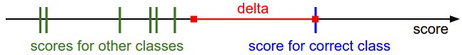
多分类的svm的损失函数是:(损失函数表明了我们的在训练集上预测的结果的不满意程度)
拿那个教材上的一个图来说明margin的用法:只有当我们的正确的分类的预测得分高于我们其他的预测得分margin个距离才能使得loss=0
除此之外,我们的还需要防止过拟合,所以我们要添加正则化,我们一般的正则化
所以我们完整的多类别svm损失函数是:
下面的代码是使用向量化和非向量化的操作分别来实现计算单个实例的代价:
def L_i(x, y, W):
  """
  unvectorized version. Compute the multiclass svm loss for a single example (x,y)
  - x is a column vector representing an image (e.g. 3073 x 1 in CIFAR-10)
    with an appended bias dimension in the 3073-rd position (i.e. bias trick)
  - y is an integer giving index of correct class (e.g. between 0 and 9 in CIFAR-10)
  - W is the weight matrix (e.g. 10 x 3073 in CIFAR-10)
  """
  delta = 1.0 # see notes about delta later in this section
  scores = W.dot(x) # scores becomes of size 10 x 1, the scores for each class
  correct_class_score = scores[y]
  D = W.shape[0] # number of classes, e.g. 10
  loss_i = 0.0
  for j in xrange(D): # iterate over all wrong classes
    if j == y:
      # skip for the true class to only loop over incorrect classes
      continue
    # accumulate loss for the i-th example
    loss_i += max(0, scores[j] - correct_class_score + delta)
  return loss_i

def L_i_vectorized(x, y, W):
  """
  A faster half-vectorized implementation. half-vectorized
  refers to the fact that for a single example the implementation contains
  no for loops, but there is still one loop over the examples (outside this function)
  """
  delta = 1.0
  scores = W.dot(x)
  # compute the margins for all classes in one vector operation
  margins = np.maximum(0, scores - scores[y] + delta)
  # on y-th position scores[y] - scores[y] canceled and gave delta. We want
  # to ignore the y-th position and only consider margin on max wrong class
  margins[y] = 0
  loss_i = np.sum(margins)
  return loss_i

def L(X, y, W):
  """
  fully-vectorized implementation :
  - X holds all the training examples as columns (e.g. 3073 x 50,000 in CIFAR-10)
  - y is array of integers specifying correct class (e.g. 50,000-D array)
  - W are weights (e.g. 10 x 3073)
  """
  # evaluate loss over all examples in X without using any for loops
  # left as exercise to reader in the assignment
对于超参数
反向传播比较的复杂,建议阅读文档:点击打开链接
当你阅读完上述的文档,你就知道SVM的梯度是多少了:对于梯度的求导维基讲的很清楚。https://en.wikipedia.org/wiki/Matrix_calculus#Scalar-by-vector_identities
得到的结果如下:
我们对于单个样本的损失函数:
求导分成下面两个:
下面开始解释函数:
首先与knn相同的是进行数据的展示,展示训练集和测试集的大小,展示每个样本的七张照片,之后我们就要将整个样本划分为三个部分,前面49,000作为训练集,之后1000个为交叉验证集,在之后再从10,000测试集中选择前面1000个为测试集。另外我们存在500个发展集(不知道什么意思)!
step1:数据的预处理,减去均值;
step2:给SVM添加全一列作为偏差项;
step3:我们要给两个函数里面添加代码(均在linear_svm.py)
注意我们首先在svm_loss_naive()里面修改一些代码完成计算梯度的部分,之后我们在svm_loss_vectorized()添加上计算loss和梯度的代码:
svm_loss_naive():这个里面的代码是在网上抄的别人的,并没有看明白!!
svm_loss_vectorized():这个里面的求loss的代码是自己写的,但是求梯度的代码也是抄的!
import numpy as np
from random import shuffle
from past.builtins import xrange

def svm_loss_naive(W, X, y, reg):
  """
  Structured SVM loss function, naive implementation (with loops).

  Inputs have dimension D, there are C classes, and we operate on minibatches
  of N examples.

  Inputs:
  - W: A numpy array of shape (D, C) containing weights.
  - X: A numpy array of shape (N, D) containing a minibatch of data.
  - y: A numpy array of shape (N,) containing training labels; y[i] = c means
    that X[i] has label c, where 0 <= c < C.
  - reg: (float) regularization strength

  Returns a tuple of:
  - loss as single float
  - gradient with respect to weights W; an array of same shape as W
  """
  dW = np.zeros(W.shape) # initialize the gradient as zero

  # compute the loss and the gradient
  num_classes = W.shape[1]
  num_train = X.shape[0]
  loss = 0.0
  for i in xrange(num_train):
    scores = X[i].dot(W)
    correct_class_score = scores[y[i]]
    for j in xrange(num_classes):
      if j == y[i]:
        continue
      margin = scores[j] - correct_class_score + 1 # note delta = 1
      if margin > 0:
        loss += margin
        dW[:,y[i]]+=-X[i,:]
        dW[:,j]+=X[i,:]
  # Right now the loss is a sum over all training examples, but we want it
  # to be an average instead so we divide by num_train.
  loss /= num_train
  dW/=num_train

  # Add regularization to the loss.
  loss += reg * np.sum(W * W)
    dW+=reg*W
  #############################################################################
  # TODO:                                                                     #
  # Compute the gradient of the loss function and store it dW.                #
  # Rather that first computing the loss and then computing the derivative,   #
  # it may be simpler to compute the derivative at the same time that the     #
  # loss is being computed. As a result you may need to modify some of the    #
  # code above to compute the gradient.                                       #
  #############################################################################


  return loss, dW


def svm_loss_vectorized(W, X, y, reg):
  """
  Structured SVM loss function, vectorized implementation.

  Inputs and outputs are the same as svm_loss_naive.
  """
  loss = 0.0
  dW = np.zeros(W.shape) # initialize the gradient as zero

  #############################################################################
  # TODO:                                                                     #
  # Implement a vectorized version of the structured SVM loss, storing the    #
  # result in loss.                                                           #
  #############################################################################
  num_train=X.shape[0]
  scores=X.dot(W)
  margin=scores-scores[np.arange(num_train),y].reshape(num_train,1)+1
  margin[np.arange(num_train),y]=0
  margin=(margin>0)*margin
  loss+=np.sum(margin)/num_train
  loss+=0.5*reg*sum(W*W)
  #############################################################################
  #                             END OF YOUR CODE                              #
  #############################################################################


  #############################################################################
  # TODO:                                                                     #
  # Implement a vectorized version of the gradient for the structured SVM     #
  # loss, storing the result in dW.                                           #
  #                                                                           #
  # Hint: Instead of computing the gradient from scratch, it may be easier    #
  # to reuse some of the intermediate values that you used to compute the     #
  # loss.                                                                     #
  #############################################################################
  margin=(margin>0)*1
    row_sum=np.sum(margin,axis=1)
    margin[np.arange(num_train,y)]=-row_sum
    dW=X.T*dot(margin)/num_train+reg*W
  #############################################################################
  #                             END OF YOUR CODE                              #
  #############################################################################

  return loss, dW
(3)SoftMax-建议先阅读文档点击打开链接
softmax是一个多项逻辑斯蒂回归,他得到的score是对类别的未正则化的log概率,它的保持不变,变得是原本的合页损失(hinge loss)变成了交叉熵损失:
或者可以写成:
。
一般我们在计算的时候会考虑到数值稳定性的问题,所以我们做如下的修改: