转载自 https://blog.csdn.net/qq_16137569/article/details/72802387 https://blog.csdn.net/xinyu3307/article/details/74643019
自己整理的,刚学,自学,欢迎批评!
目录
猫狗大战数据集准备
Cats vs. Dogs(猫狗大战)是Kaggle大数据竞赛某一年的一道赛题,利用给定的数据集,用算法实现猫和狗的识别。
数据集可以从Kaggle官网上下载:
- 12500张cat
- 12500张dog
https://www.kaggle.com/c/dogs-vs-cats
或者在这里下载 https://blog.csdn.net/qq_20073741/article/details/81233326
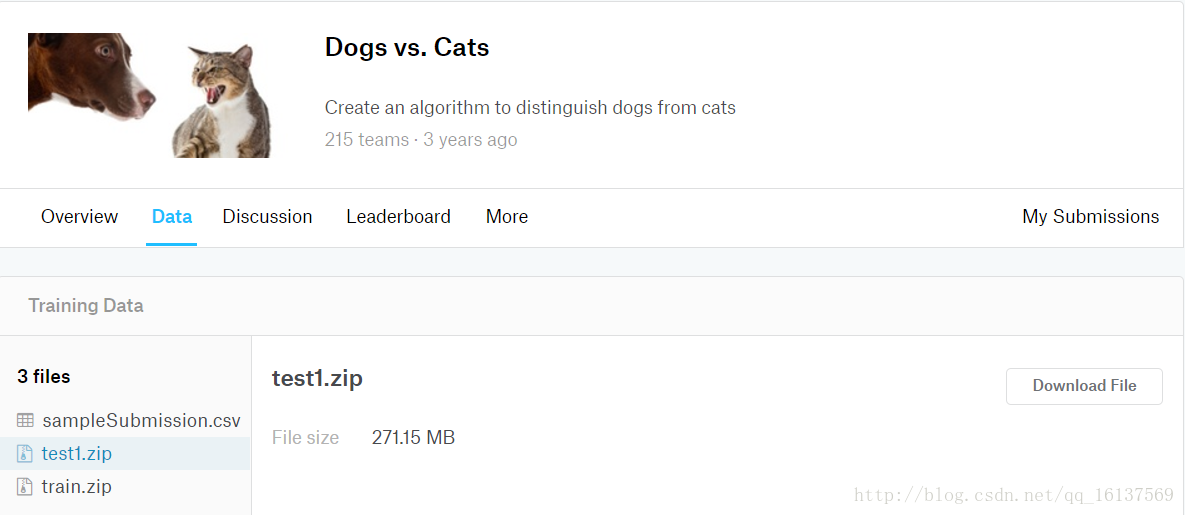
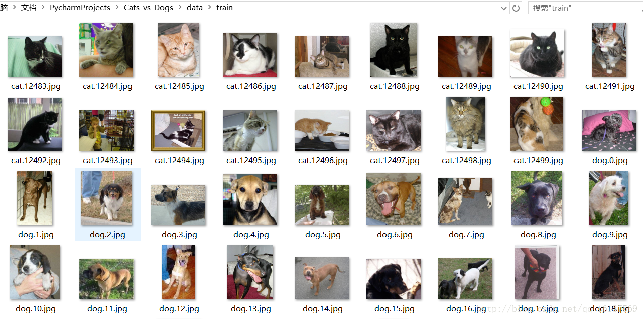
数据集由训练数据和测试数据组成,训练数据包含猫和狗各12500张图片,测试数据包含12500张猫和狗的图片。
首先在Pycharm上新建Cats_vs_Dogs工程,工程目录结构为:
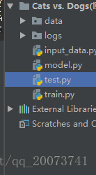
data文件夹下包含test和train两个子文件夹,分别用于存放测试数据和训练数据,从官网上下载的数据直接解压到相应的文件夹下即可logs文件夹用于存放我们训练时的模型结构以及训练参数input_data.py负责实现读取数据,生成批次(batch)model.py负责实现我们的神经网络模型training.py负责实现模型的训练以及评估- test.py 负责我们想测试的图片
接下来分成数据读取、模型构造、模型训练、测试模型四个部分来讲。源码从文章末尾的链接下载。
训练数据的读取——input_data.py
导入模块
tensorflow和numpy不用多说,其中os模块包含操作系统相关的功能,可以处理文件和目录这些我们日常手动需要做的操作。因为我们需要获取test目录下的文件,所以要导入os模块。
import tensorflow as tf
import numpy as np
import os
生成图片路径和标签的List
# 获取文件路径和标签
def get_files(file_dir):
    # file_dir: 文件夹路径
    # return: 乱序后的图片和标签

    cats = []
    label_cats = []
    dogs = []
    label_dogs = []
    # 载入数据路径并写入标签值
    for file in os.listdir(file_dir):
        name = file.split(sep='.')
        if name[0] == 'cat':
            cats.append(file_dir + file)
            label_cats.append(0)
        else:
            dogs.append(file_dir + file)
            label_dogs.append(1)
    print("There are %d cats\nThere are %d dogs" % (len(cats), len(dogs)))

    # 打乱文件顺序
    image_list = np.hstack((cats, dogs))   #a=[1,2,3] b=[4,5,6] print(np.hstack((a,b)))
                                           #输出:[1 2 3 4 5 6 ]
    label_list = np.hstack((label_cats, label_dogs))
    temp = np.array([image_list, label_list])
    temp = temp.transpose()     # 转置
    np.random.shuffle(temp)     ##利用shuffle打乱顺序

    ##从打乱的temp中再取出list(img和lab)
    image_list = list(temp[:, 0])
    label_list = list(temp[:, 1])
    label_list = [int(i) for i in label_list]  #字符串类型转换为int类型

return image_list, label_list 函数get_files(file_dir)的功能是获取给定路径file_dir下的所有的训练数据(包括图片和标签),以list的形式返回。
由于训练数据前12500张是猫,后12500张是狗,如果直接按这个顺序训练,训练效果可能会受影响(我自己猜的),所以需要将顺序打乱,至于是读取数据的时候乱序还是训练的时候乱序可以自己选择(视频里说在这里乱序速度比较快)。因为图片和标签是一一对应的,所以要整合到一起乱序。
这里先用np.hstack()方法将猫和狗图片和标签整合到一起,得到image_list和label_list,hstack((a,b))的功能是将a和b以水平的方式连接,比如原来cats和dogs是长度为12500的向量,执行了hstack(cats, dogs)后,image_list的长度为25000,同理label_list的长度也为25000。接着将一一对应的image_list和label_list再合并一次。temp的大小是2×25000,经过转置(变成25000×2),然后使用np.random.shuffle()方法进行乱序。
最后从temp中分别取出乱序后的image_list和label_list列向量,作为函数的返回值。这里要注意,因为label_list里面的数据类型是字符串类型,所以加上label_list = [int(i) for i in label_list]这么一行将其转为int类型。
生成Batch
将上面生成的List传入get_batch() ,转换类型,产生一个输入队列queue,因为img和lab是分开的,所以使用tf.train.slice_input_producer(),然后用tf.read_file()从队列中读取图像
# 生成相同大小的批次
def get_batch(image, label, image_W, image_H, batch_size, capacity):
    # image, label: 要生成batch的图像和标签list
    # image_W, image_H: 图片的宽高
    # batch_size: 每个batch有多少张图片
    # capacity: 队列容量,一个队列最大多少
    # return: 图像和标签的batch

    # 将python.list类型转换成tf能够识别的格式
    image = tf.cast(image, tf.string)
    label = tf.cast(label, tf.int32)

    # 生成队列 ,将image 和 label 放倒队列里
    input_queue = tf.train.slice_input_producer([image, label])

    image_contents = tf.read_file(input_queue[0])  ## 读取图片的全部信息
    label = input_queue[1]
    #将图像解码,不同类型的图像不能混在一起,要么只用jpeg,要么只用png等
    ## 把图片解码,channels =3 为彩色图片, r,g ,b  黑白图片为 1 ,也可以理解为图片的厚度
    image = tf.image.decode_jpeg(image_contents, channels=3)

    # 统一图片大小
    # 将图片以图片中心进行裁剪或者扩充为 指定的image_W,image_H
    # image = tf.image.resize_image_with_crop_or_pad(image, image_W, image_H)
    # 我的方法

    image = tf.image.resize_images(image, [image_H, image_W], method=tf.image.ResizeMethod.NEAREST_NEIGHBOR)     #最近邻插值方法
    image = tf.cast(image, tf.float32)          #string类型转换为float
    # image = tf.image.per_image_standardization(image)   # 对数据进行标准化,标准化,就是减
                                                           #去它的均值,除以他的方差

    # 生成批次  num_threads 有多少个线程根据电脑配置设置  capacity 队列中 最多容纳图片的个数
     #tf.train.shuffle_batch 打乱顺序,
    image_batch, label_batch = tf.train.batch([image, label],
                                              batch_size=batch_size,
                                              num_threads=64,   # 线程
                                              capacity=capacity)

    # 这两行多余? 重新排列label,行数为[batch_size],有兴趣可以试试看
    # label_batch = tf.reshape(label_batch, [batch_size])


return image_batch, label_batch 函数get_batch()用于将图片分批次,因为一次性将所有25000张图片载入内存不现实也不必要,所以将图片分成不同批次进行训练。这里传入的image和label参数就是函数get_files()返回的image_list和label_list,是python中的list类型,所以需要将其转为TensorFlow可以识别的tensor格式。
这里使用队列来获取数据,因为队列操作牵扯到线程,我自己对这块也不懂,,所以只从大体上理解了一下,想要系统学习可以去官方文档看看,这里引用了一张图解释。

我认为大体上可以这么理解:每次训练时,从队列中取一个batch送到网络进行训练,然后又有新的图片从训练库中注入队列,这样循环往复。队列相当于起到了训练库到网络模型间数据管道的作用,训练数据通过队列送入网络。(我也不确定这么理解对不对,欢迎指正)
继续看程序,我们使用slice_input_producer()来建立一个队列,将image和label放入一个list中当做参数传给该函数。然后从队列中取得image和label,要注意,用read_file()读取图片之后,要按照图片格式进行解码。本例程中训练数据是jpg格式的,所以使用decode_jpeg()解码器,如果是其他格式,就要用其他解码器,具体可以从官方API中查询。注意decode出来的数据类型是uint8,之后模型卷积层里面conv2d()要求输入数据为float32类型,所以如果删掉标准化步骤之后需要进行类型转换。
因为训练库中图片大小是不一样的,所以还需要将图片裁剪成相同大小(img_W和img_H)。视频中是用resize_image_with_crop_or_pad()方法来裁剪图片,这种方法是从图像中心向四周裁剪,如果图片超过规定尺寸,最后只会剩中间区域的一部分,可能一只狗只剩下躯干,头都不见了,用这样的图片训练结果肯定会受到影响。所以这里我稍微改动了一下,使用resize_images()对图像进行缩放,而不是裁剪,采用NEAREST_NEIGHBOR插值方法(其他几种插值方法出来的结果图像是花的,具体原因不知道)。
缩放之后视频中还进行了per_image_standardization (标准化)步骤,但加了这步之后,得到的图片是花的,虽然各个通道单独提出来是正常的,三通道一起就不对了,删了标准化这步结果正常,所以这里把标准化步骤注释掉了。
然后用tf.train.batch()方法获取batch,还有一种方法是tf.train.shuffle_batch(),因为之前我们已经乱序过了,这里用普通的batch()就好。视频中获取batch后还对label进行了一下reshape()操作,在我看来这步是多余的,从batch()方法中获取的大小已经符合我们的要求了,注释掉也没什么影响,能正常获取图片。
最后将得到的image_batch和label_batch返回。image_batch是一个4D的tensor,[batch, width, height, channels],label_batch是一个1D的tensor,[batch]。
可以用下面的代码测试获取图片是否成功,因为之前将图片转为float32了,因此这里imshow()出来的图片色彩会有点奇怪,因为本来imshow()是显示uint8类型的数据(灰度值在uint8类型下是0~255,转为float32后会超出这个范围,所以色彩有点奇怪),不过这不影响后面模型的训练。
测试
变量初始化,每批2张图,尺寸208x208,设置好自己的图像路径
# TEST
import matplotlib.pyplot as plt

BATCH_SIZE = 2
CAPACITY = 256
IMG_W = 208
IMG_H = 208

train_dir = "data\\train\\"
 #调用前面的两个函数,生成batch
image_list, label_list = get_files(train_dir)
image_batch, label_batch = get_batch(image_list, label_list, IMG_W, IMG_H, BATCH_SIZE, CAPACITY)

#开启会话session,利用tf.train.Coordinator()和tf.train.start_queue_runners(coord=coord)来监控队列(这里有个问题:官网的start_queue_runners()是有两个参数的,sess和coord,但是在这里加上sess的话会报错)。
利用try——except——finally结构来执行队列操作(官网推荐的方法),避免程序卡死什么的。i<2执行两次队列操作,每一次取出2张图放进batch里面,然后imshow出来看看效果

with tf.Session() as sess:
    i = 0
    ##  Coordinator  和 start_queue_runners 监控 queue 的状态,不停的入队出队1
    coord = tf.train.Coordinator()
    threads = tf.train.start_queue_runners(coord=coord)
    try:
        while not coord.should_stop() and i < 1:
            img, label = sess.run([image_batch, label_batch])

            for j in np.arange(BATCH_SIZE):
                print("label: %d" % label[j])
                plt.imshow(img[j, :, :, :])
                plt.show()
            i += 1
   #队列中没有数据
    except tf.errors.OutOfRangeError:
        print("done!")
    finally:
        coord.request_stop()
    coord.join(threads)
卷积神经网络模型的构造——model.py
关于神经网络模型不想说太多,视频中使用的模型是仿照TensorFlow的官方例程cifar-10的网络结构来写的。就是两个卷积层(每个卷积层后加一个池化层),两个全连接层,最后一个softmax输出分类结果。
简单的卷积神经网络
-
一个简单的卷积神经网络,卷积+池化层x2,全连接层x2,最后一个softmax层做分类。
推理函数:def inference(images, batch_size, n_classes): - 输入参数:
images,image batch、4D tensor、tf.float32、[batch_size, width, height, channels] - 返回参数:
logits, float、 [batch_size, n_classes] -
import tensorflow as tf

# 结构
# conv1   卷积层 1
# pooling1_lrn  池化层 1
# conv2  卷积层 2
# pooling2_lrn 池化层 2
# local3 全连接层 1
# local4 全连接层 2
# softmax 全连接层 3

def inference(images, batch_size, n_classes):
    # conv1, shape = [kernel_size, kernel_size, channels, kernel_numbers]
    #卷积层1 16个3x3的卷积核(3通道),padding=’SAME’,表示padding后卷积的图与原图尺寸一致,激活函数relu()
    with tf.variable_scope("conv1") as scope:
        weights = tf.get_variable("weights",
                                  shape=[3, 3, 3, 16],
                                  dtype=tf.float32,
                                  initializer=tf.truncated_normal_initializer(stddev=0.1, dtype=tf.float32))
        biases = tf.get_variable("biases",
                                 shape=[16],
                                 dtype=tf.float32,
                                 initializer=tf.constant_initializer(0.1))
        conv = tf.nn.conv2d(images, weights, strides=[1, 1, 1, 1], padding="SAME")
        pre_activation = tf.nn.bias_add(conv, biases)
        conv1 = tf.nn.relu(pre_activation, name="conv1")

    # pool1 && norm1
    # 池化层1 3x3最大池化,步长strides为2,池化后执行lrn()操作,局部响应归一化,对训练有利。
    with tf.variable_scope("pooling1_lrn") as scope:
        pool1 = tf.nn.max_pool(conv1, ksize=[1, 3, 3, 1], strides=[1, 2, 2, 1],
                               padding="SAME", name="pooling1")
        norm1 = tf.nn.lrn(pool1, depth_radius=4, bias=1.0, alpha=0.001/9.0,
                          beta=0.75, name='norm1')

    # conv2
    #卷积层2 16个3x3的卷积核(16通道),padding=’SAME’,表示padding后卷积的图与原图尺寸一致,激活函数relu()
    with tf.variable_scope("conv2") as scope:
        weights = tf.get_variable("weights",
                                  shape=[3, 3, 16, 16],
                                  dtype=tf.float32,
                                  initializer=tf.truncated_normal_initializer(stddev=0.1, dtype=tf.float32))
        biases = tf.get_variable("biases",
                                 shape=[16],
                                 dtype=tf.float32,
                                 initializer=tf.constant_initializer(0.1))
        conv = tf.nn.conv2d(norm1, weights, strides=[1, 1, 1, 1], padding="SAME")
        pre_activation = tf.nn.bias_add(conv, biases)
        conv2 = tf.nn.relu(pre_activation, name="conv2")

    # pool2 && norm2
    #池化层2 3x3最大池化,步长strides为2,池化后执行lrn()操作,
    with tf.variable_scope("pooling2_lrn") as scope:
        pool2 = tf.nn.max_pool(conv2, ksize=[1, 3, 3, 1], strides=[1, 2, 2, 1],
                               padding="SAME", name="pooling2")
        norm2 = tf.nn.lrn(pool2, depth_radius=4, bias=1.0, alpha=0.001/9.0,
                          beta=0.75, name='norm2')

    # full-connect1
    #全连接层1 128个神经元,将之前pool层的输出reshape成一行,激活函数relu()
    with tf.variable_scope("fc1") as scope:
        reshape = tf.reshape(norm2, shape=[batch_size, -1])
        dim = reshape.get_shape()[1].value
        weights = tf.get_variable("weights",
                                  shape=[dim, 128],
                                  dtype=tf.float32,
                                  initializer=tf.truncated_normal_initializer(stddev=0.005, dtype=tf.float32))
        biases = tf.get_variable("biases",
                                 shape=[128],
                                 dtype=tf.float32,
                                 initializer=tf.constant_initializer(0.1))
        fc1 = tf.nn.relu(tf.matmul(reshape, weights) + biases, name="fc1")

    # full_connect2
    #全连接层2 128个神经元,激活函数relu()
    with tf.variable_scope("fc2") as scope:
        weights = tf.get_variable("weights",
                                  shape=[128, 128],
                                  dtype=tf.float32,
                                  initializer=tf.truncated_normal_initializer(stddev=0.005, dtype=tf.float32))
        biases = tf.get_variable("biases",
                                 shape=[128],
                                 dtype=tf.float32,
                                 initializer=tf.constant_initializer(0.1))
        fc2 = tf.nn.relu(tf.matmul(fc1, weights) + biases, name="fc2")

    # softmax
    #Softmax回归层 将前面的FC层输出,做一个线性回归,计算出每一类的得分,在这里是2类,所以这个层输出的是两个得分
    with tf.variable_scope("softmax_linear") as scope:
       #weights = tf.get_variable("softmax_linear",有一个链接是写成这样子的,大家可以试试
        weights = tf.get_variable("weights",
                                  shape=[128, n_classes],
                                  dtype=tf.float32,
                                  initializer=tf.truncated_normal_initializer(stddev=0.005, dtype=tf.float32))
        biases = tf.get_variable("biases",
                                 shape=[n_classes],
                                 dtype=tf.float32,
                                 initializer=tf.constant_initializer(0.1))
        softmax_linear = tf.add(tf.matmul(fc2, weights), biases, name="softmax_linear")
        softmax_linear = tf.nn.softmax(softmax_linear)
    return softmax_linear
发现程序里面有很多with tf.variable_scope("name")的语句,这其实是TensorFlow中的变量作用域机制,目的是有效便捷地管理需要的变量。
变量作用域机制在TensorFlow中主要由两部分组成:
tf.get_variable(<name>, <shape>, <initializer>): 创建一个变量tf.variable_scope(<scope_name>): 指定命名空间
如果需要共享变量,需要通过reuse_variables()方法来指定,详细的例子去官方文档中看就好了。(链接在博客参考部分)
loss计算
将网络计算得出的每类得分与真实值进行比较,得出一个loss损失值,这个值代表了计算值与期望值的差距。这里使用的loss函数是交叉熵。一批loss取平均数。最后调用了summary.scalar()记录下这个标量数据,在TensorBoard中进行可视化。
函数:def losses(logits, labels):
- 传入参数:logits,网络计算输出值。labels,真实值,在这里是0或者1
- 返回参数:loss,损失值
#loss计算
def losses(logits, labels):
    with tf.variable_scope("loss") as scope:
        cross_entropy = tf.nn.sparse_softmax_cross_entropy_with_logits(logits=logits,
                                                                       labels=labels, name="xentropy_per_example")
        loss = tf.reduce_mean(cross_entropy, name="loss")
        tf.summary.scalar(scope.name + "loss", loss)
    return loss
loss损失值优化
目的就是让loss越小越好,使用的是AdamOptimizer优化器
函数:def trainning(loss, learning_rate):
- 输入参数:loss。learning_rate,学习速率。
- 返回参数:train_op,训练op,这个参数要输入sess.run中让模型去训练
#loss损失值优化
def trainning(loss, learning_rate):
    with tf.name_scope("optimizer"):
        optimizer = tf.train.AdamOptimizer(learning_rate=learning_rate)
        global_step = tf.Variable(0, name="global_step", trainable=False)
        train_op = optimizer.minimize(loss, global_step=global_step)
    return train_op
评价/准确率计算
计算出平均准确率来评价这个模型,在训练过程中按批次计算(每隔N步计算一次),可以看到准确率的变换情况。
函数:def evaluation(logits, labels):
- 输入参数:logits,网络计算值。labels,标签,也就是真实值,在这里是0或者1。
- 返回参数:accuracy,当前step的平均准确率,也就是在这些batch中多少张图片被正确分类了
#评价/准确率计算
def evaluation(logits, labels):
    with tf.variable_scope("accuracy") as scope:
        correct = tf.nn.in_top_k(logits, labels, 1)
        correct = tf.cast(correct, tf.float16)
        accuracy = tf.reduce_mean(correct)
        tf.summary.scalar(scope.name + "accuracy", accuracy)
return accuracy 函数losses(logits, labels)用于计算训练过程中的loss,这里输入参数logtis是函数inference()的输出,代表图片对猫和狗的预测概率,labels则是图片对应的标签。
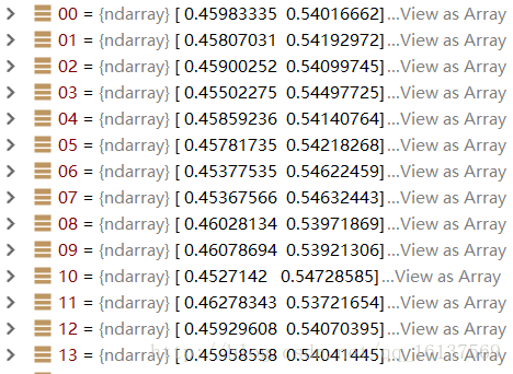
通过在程序中设置断点,查看logtis的值,结果如下图所示,根据这个就很好理解了,一个数值代表属于猫的概率,一个数值代表属于狗的概率,两者的和为1。
而函数tf.nn.sparse_sotfmax_cross_entropy_with_logtis从名字就很好理解,是将稀疏表示的label与输出层计算出来结果做对比。然后因为训练的时候是16张图片一个batch,所以再用tf.reduce_mean求一下平均值,就得到了这个batch的平均loss。
training(loss, learning_rate)就没什么好说的了,loss是训练的loss,learning_rate是学习率,使用AdamOptimizer优化器来使loss朝着变小的方向优化。
evaluation(logits, labels)功能是在训练过程中实时监测验证数据的准确率,达到反映训练效果的作用。
模型训练-train.py
导入文件
import os
import numpy as np
import tensorflow as tf
import input_data
import model
变量声明
N_CLASSES = 2 # 2个输出神经元,[1,0] 或者 [0,1]猫和狗的概率
IMG_W = 208  # resize图像,太大的话训练时间久
IMG_H = 208
BATCH_SIZE = 16
CAPACITY = 2000
MAX_STEP = 10000 # 一般大于10K
learning_rate = 0.0001 # 一般小于0.0001
获取批次batch
train_dir = './data/train/'
logs_train_dir = './logs/train/'    #这个目录会自动生成

 # 获取图片和标签集
train, train_label = input_data.get_files(train_dir)
 ## 生成批次
train_batch,train_label_batch=input_data.get_batch(train,
                                train_label,
                                IMG_W,
                                IMG_H,
                                BATCH_SIZE,
                                CAPACITY)
操作定义
#操作定义  进入模型
train_logits = model.inference(train_batch, BATCH_SIZE, N_CLASSES)
#获取loss
train_loss = model.losses(train_logits, train_label_batch)
#训练
train_op = model.trainning(train_loss, learning_rate)
#获取准确率
train__acc = model.evaluation(train_logits, train_label_batch)
合并summary
summary_op = tf.summary.merge_all() #这个是log汇总记录
#产生一个会话
sess = tf.Session()
#产生一个writer来写log文件
train_writer = tf.summary.FileWriter(logs_train_dir, sess.graph)
 #产生一个saver来存储训练好的模型
saver = tf.train.Saver()
#所有节点初始化
sess.run(tf.global_variables_initializer())

#队列监控
coord = tf.train.Coordinator()
threads = tf.train.start_queue_runners(sess=sess, coord=coord)
进行batch的训练
#进行batch的训练
try:
    #执行MAX_STEP步的训练,一步一个batch
    for step in np.arange(MAX_STEP):
        if coord.should_stop():
                break
        #启动以下操作节点,有个疑问,为什么train_logits在这里没有开启?
        _, tra_loss, tra_acc = sess.run([train_op, train_loss, train__acc])
        #每隔50步打印一次当前的loss以及acc,同时记录log,写入writer
        if step % 50 == 0:
            print('Step %d, train loss = %.2f, train accuracy = %.2f%%' %(step, tra_loss, tra_acc*100.0))
            summary_str = sess.run(summary_op)
            train_writer.add_summary(summary_str, step)
        #每隔2000步,保存一次训练好的模型
        if step % 2000 == 0 or (step + 1) == MAX_STEP:
            checkpoint_path = os.path.join(logs_train_dir, 'model.ckpt')
            saver.save(sess, checkpoint_path, global_step=step)

except tf.errors.OutOfRangeError:
    print('Done training -- epoch limit reached')
finally:
    coord.request_stop()
测试代码-test.py
导入模块
import tensorflow as tf
from PIL import Image
import matplotlib.pyplot as plt
import input_data
import numpy as np
import model
import os
获取一张图片
函数:def get_one_image(train):
输入参数:train,训练图片的路径
返回参数:image,从训练图片中随机抽取一张图片
-
#从指定目录中选取一张图片
def get_one_image(train):
    files = os.listdir(train)
    n = len(files)
    n = len(train)
    ind = np.random.randint(0,n)
    img_dir = os.path.join(train,files[ind])
    image = Image.open(img_dir)
    plt.imshow(image)
    plt.show()
    image = image.resize([208, 208])
    image = np.array(image)
    return image
测试图片
函数:
def evaluate_one_image(): -
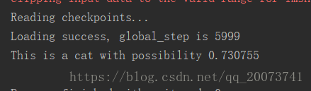
#测试图片
def evaluate_one_image():
    #存放我们想测试的图片集
    train = './data/test/'
    image_array = get_one_image(train)
with tf.Graph().as_default():
       BATCH_SIZE = 1   # 因为只读取一副图片 所以batch 设置为1
       N_CLASSES = 2    ## 2个输出神经元,[1,0] 或者 [0,1]猫和狗的概率
       # 转化图片格式
       image = tf.cast(image_array, tf.float32)
       # 图片标准化
       image = tf.image.per_image_standardization(image)
       # 图片原来是三维的 [208, 208, 3] 重新定义图片形状 改为一个4D  四维的 tensor
       image = tf.reshape(image, [1, 208, 208, 3])
       logit = model.inference(image, BATCH_SIZE, N_CLASSES)
       # 因为 inference 的返回没有用激活函数,所以在这里对结果用softmax 激活
       logit = tf.nn.softmax(logit)
       # 用最原始的输入数据的方式向模型输入数据 placeholder
       x = tf.placeholder(tf.float32, shape=[208, 208, 3])

       # 我门存放模型的路径
       logs_train_dir = './Logs/train'

        # 定义saver
       saver = tf.train.Saver()

       with tf.Session() as sess:

           print("Reading checkpoints...")
           # 将模型加载到sess 中
           ckpt = tf.train.get_checkpoint_state(logs_train_dir)
           if ckpt and ckpt.model_checkpoint_path:
               global_step = ckpt.model_checkpoint_path.split('/')[-1].split('-')[-1]
               saver.restore(sess, ckpt.model_checkpoint_path)
               print('Loading success, global_step is %s' % global_step)
           else:
               print('No checkpoint file found')

           prediction = sess.run(logit, feed_dict={x: image_array})
           max_index = np.argmax(prediction)
           if max_index==0:
               print('This is a cat with possibility %.6f' %prediction[:, 0])
           else:
               print('This is a dog with possibility %.6f' %prediction[:, 1])