在学习机器学习算法的过程中，我们经常需要数据来验证算法，调试参数。但是找到一组十分合适某种特定算法类型的数据样本却不那么容易。还好numpy, scikit-learn都提供了随机数据生成的功能，我们可以自己生成适合某一种模型的数据，用随机数据来做清洗，归一化，转换，然后选择模型与算法做拟合和预测。下面对scikit-learn和numpy生成数据样本的方法做一个总结。

1. numpy随机数据生成API

　　　　numpy比较适合用来生产一些简单的抽样数据。API都在random类中，常见的API有：

　　　　1) rand(d0, d1, …, dn) 用来生成d0xd1x…dn维的数组。数组的值在[0,1]之间

　　　　例如：np.random.rand(3,2,2)，输出如下3x2x2的数组

array([[[ 0.49042678,  0.60643763],
        [ 0.18370487,  0.10836908]],

       [[ 0.38269728,  0.66130293],
        [ 0.5775944 ,  0.52354981]],

       [[ 0.71705929,  0.89453574],
        [ 0.36245334,  0.37545211]]])　　

　　　　2) randn((d0, d1, …, dn), 也是用来生成d0xd1x…dn维的数组。不过数组的值服从N(0,1)的标准正态分布。

　　　　例如：np.random.randn(3,2)，输出如下3x2的数组，这些值是N(0,1)的抽样数据。

array([[-0.5889483 , -0.34054626],
       [-2.03094528, -0.21205145],
       [-0.20804811, -0.97289898]])

如果需要服从N(μ,σ2)’>N(μ,σ2)N(μ,σ2)即可，例如：

例如：2*np.random.randn(3,2) + 1，输出如下3x2的数组，这些值是N(1,4)的抽样数据。

array([[ 2.32910328, -0.677016  ],
       [-0.09049511,  1.04687598],
       [ 2.13493001,  3.30025852]])

3)randint(low[, high, size])，生成随机的大小为size的数据，size可以为整数，为矩阵维数，或者张量的维数。值位于半开区间 [low, high)。

　　　　例如：np.random.randint(3, size=[2,3,4])返回维数维2x3x4的数据。取值范围为最大值为3的整数。

　　　　　　array([[[2, 1, 2, 1],
　　　　　　　　　　[0, 1, 2, 1],
　　　　　　　　　　[2, 1, 0, 2]],

　　　　　　　　　　[[0, 1, 0, 0],
　　　　　　　　　　[1, 1, 2, 1],
　　　　　　　　　　[1, 0, 1, 2]]])

　　　　再比如： np.random.randint(3, 6, size=[2,3]) 返回维数为2x3的数据。取值范围为[3,6).

　　　　　　array([[4, 5, 3],
　　　　　　　　[3, 4, 5]])

　　　　4) random_integers(low[, high, size]),和上面的randint类似，区别在与取值范围是闭区间[low, high]。

　　　　5) random_sample([size]), 返回随机的浮点数，在半开区间 [0.0, 1.0)。如果是其他区间[a,b),可以加以转换(b - a) * random_sample([size]) + a

　　　　例如： (5-2)*np.random.random_sample(3)+2 返回[2,5)之间的3个随机数。

　　　　　　array([ 2.87037573,  4.33790491,  2.1662832 ])

2. scikit-learn随机数据生成API介绍

　　　　scikit-learn生成随机数据的API都在datasets类之中，和numpy比起来，可以用来生成适合特定机器学习模型的数据。常用的API有：

　　　　1) 用make_regression 生成回归模型的数据

　　　　2) 用make_hastie_10_2，make_classification或者make_multilabel_classification生成分类模型数据

　　　　3) 用make_blobs生成聚类模型数据

　　　　4) 用make_gaussian_quantiles生成分组多维正态分布的数据

3. scikit-learn随机数据生成实例

3.1 回归模型随机数据

 　　　　这里我们使用make_regression生成回归模型数据。几个关键参数有n_samples（生成样本数）， n_features（样本特征数），noise（样本随机噪音）和coef（是否返回回归系数）。例子代码如下：

import numpy as np
import matplotlib.pyplot as plt
%matplotlib inline
from sklearn.datasets.samples_generator import make_regression
# X为样本特征，y为样本输出， coef为回归系数，共1000个样本，每个样本1个特征
X, y, coef =make_regression(n_samples=1000, n_features=1,noise=10, coef=True)
# 画图
plt.scatter(X, y,  color='black')
plt.plot(X, X*coef, color='blue',
         linewidth=3)

plt.xticks(())
plt.yticks(())

plt.show()

输出的图如下：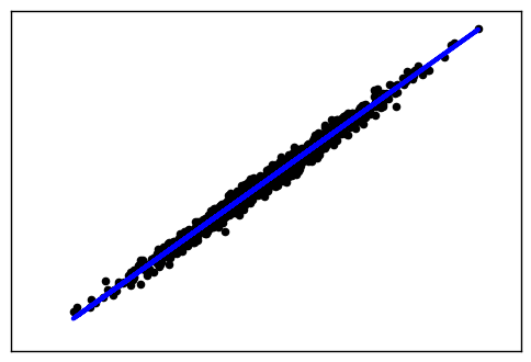

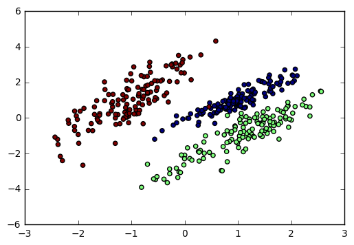
3.2 分类模型随机数据

　　　　这里我们用make_classification生成三元分类模型数据。几个关键参数有n_samples（生成样本数）， n_features（样本特征数）， n_redundant（冗余特征数）和n_classes（输出的类别数），例子代码如下：

import numpy as np
import matplotlib.pyplot as plt
%matplotlib inline
from sklearn.datasets.samples_generator import make_classification
# X1为样本特征，Y1为样本类别输出， 共400个样本，每个样本2个特征，输出有3个类别，没有冗余特征，每个类别一个簇
X1, Y1 = make_classification(n_samples=400, n_features=2, n_redundant=0,
                             n_clusters_per_class=1, n_classes=3)
plt.scatter(X1[:, 0], X1[:, 1], marker='o', c=Y1)
plt.show()

输出的图如下：

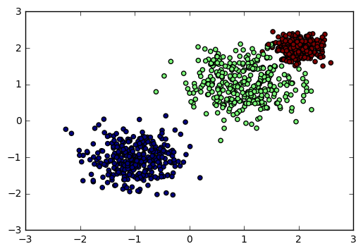
3.3 聚类模型随机数据

　　　　这里我们用make_blobs生成聚类模型数据。几个关键参数有n_samples（生成样本数）， n_features（样本特征数），centers(簇中心的个数或者自定义的簇中心)和cluster_std（簇数据方差，代表簇的聚合程度）。例子如下：

import numpy as np
import matplotlib.pyplot as plt
%matplotlib inline
from sklearn.datasets.samples_generator import make_blobs
# X为样本特征，Y为样本簇类别， 共1000个样本，每个样本2个特征，共3个簇，簇中心在[-1,-1], [1,1], [2,2]， 簇方差分别为[0.4, 0.5, 0.2]
X, y = make_blobs(n_samples=1000, n_features=2, centers=[[-1,-1], [1,1], [2,2]], cluster_std=[0.4, 0.5, 0.2])
plt.scatter(X[:, 0], X[:, 1], marker='o', c=y)
plt.show()

输出的图如下：

3.4 分组正态分布混合数据

　　　　我们用make_gaussian_quantiles生成分组多维正态分布的数据。几个关键参数有n_samples（生成样本数）， n_features（正态分布的维数），mean（特征均值）， cov（样本协方差的系数）， n_classes（数据在正态分布中按分位数分配的组数）。 例子如下：

import numpy as np
import matplotlib.pyplot as plt
%matplotlib inline
from sklearn.datasets import make_gaussian_quantiles
#生成2维正态分布，生成的数据按分位数分成3组，1000个样本,2个样本特征均值为1和2，协方差系数为2
X1, Y1 = make_gaussian_quantiles(n_samples=1000, n_features=2, n_classes=3, mean=[1,2],cov=2)
plt.scatter(X1[:, 0], X1[:, 1], marker='o', c=Y1)

输出图如下

2. plot 画图相关

在matplotlib中，整个图像为一个Figure对象。在Figure对象中可以包含一个或者多个Axes对象。每个Axes(ax)对象都是一个拥有自己坐标系统的绘图区域。在pyplot中，画纸的概念对应的就是Axes/Subplot。

plt.subplot(221) # 第一行的左图
plt.subplot(222) # 第一行的右图
plt.subplot(212) # 第二整行
plt.show()

3. 降维

可以将流形学习方法分为线性的和非线性的两种，线性的流形学习方法如我们熟知的主成份分析（PCA），非线性的流形学习方法如等距映射（Isomap）、拉普拉斯特征映射（Laplacian eigenmaps，LE）、局部线性嵌入(Locally-linear embedding，LLE)。一图概括所有。

t-SNE算是比较新的一种方法，也是效果比较好的一种方法.该方法是流形（非线性）数据降维的经典，从发表至今鲜有新的降维方法能全面超越。该方法相比PCA等线性方法能有效将数据投影到低维空间并保持严格的分割界面；缺点是计算复杂度大，一般推荐先线性降维然后再用tSNE降维.

4.：使用K-Means算法检测DGA域名

1..数据搜集和数据清洗 加载alexa前100的域名作为白样本，标记为0；分别加载cryptolocker 和post-tovar-goz家族的DGA域名，分别标记为2和3：

x1_domain_list = load_alexa("../data/dga/top-100.csv") 
x2_domain_list = load_dga("../data/dga/dga-cryptolocke-50.txt") 
x3_domain_list = load_dga("../data/dga/dga-post-tovar-goz-50.txt") 
x_domain_list=np.concatenate((x1_domain_list, x2_domain_list,x3_domain_list)) 
y1=[0]*len(x1_domain_list) 
y2=[1]*len(x2_domain_list) 
y3=[2]*len(x3_domain_list) 
y=np.concatenate((y1, y2,y3))

 ```

####2.特征化 
以2-gram分隔域名，切割单元为字符，以整个数据集合的2-gram结 果作为词汇表并进行映射，得到特征化的向量：


2-gram分词

cv = CountVectorizer(ngram_range=(2, 2), decode_error=”ignore”, token_pattern=r”\w”, min_df=1)
x= cv.fit_transform(x_domain_list).toarray()

2-gram分词也是一种最大概率分词，只不过在计算一个词概率的时候，它不光考虑自己，还会考虑它的前驱。
我们需要两个字典。第一个字典记录词wi
出现的频次，第二个字典记录词对儿<wj,wi>共同出现的频次。有这两份字典，我们就可以计算出条件概率p(wi|wj)=p(wi,wj)/p(wj)

####3.训练样本 实例化K-Means算法：
model=KMeans(n_clusters=2, random_state=random_state) 
y_pred = model.fit_predict(x)

#####4.效果验证 使用TSNE将高维向量降维，便于作图：
tsne = TSNE(learning_rate=100)
 x=tsne.fit_transform(x)

可视化聚类效果（见图10-5），其中DGA域名使用符号“×”标识：
for i,label in enumerate(x):   
 x1,x2=x[i]    if y_pred[i] == 1:     
else:       
lt.scatter(x1, x2,marker='x')    
plt.show()

总的代码

# -*- coding:utf-8 -*-

import sys
import re
import numpy as np
from sklearn.externals import joblib
import csv
import matplotlib.pyplot as plt
import os
from sklearn.feature_extraction.text import CountVectorizer
from sklearn import cross_validation
import os
from sklearn.naive_bayes import GaussianNB
from sklearn.cluster import KMeans
from sklearn.manifold import TSNE


#####3处理域名的最小长度
MIN_LEN=10
##########随机程度
random_state = 170
def load_alexa(filename):
    domain_list=[]
    csv_reader = csv.reader(open(filename))
    for row in csv_reader:
        domain=row[1]
        if domain >= MIN_LEN:
            domain_list.append(domain)
    return domain_list

def domain2ver(domain):
    ver=[]
    for i in range(0,len(domain)):
        ver.append([ord(domain[i])])
    return ver


def load_dga(filename):
    domain_list=[]
    #xsxqeadsbgvpdke.co.uk,Domain used by Cryptolocker - Flashback DGA for 13 Apr 2017,2017-04-13,
    # http://osint.bambenekconsulting.com/manual/cl.txt
    with open(filename) as f:
        for line in f:
            domain=line.split(",")[0]
            if domain >= MIN_LEN:
                domain_list.append(domain)
    return  domain_list
    def nb_dga():
    x1_domain_list = load_alexa("../data/top-1000.csv")
    x2_domain_list = load_dga("../data/dga-cryptolocke-1000.txt")
    x3_domain_list = load_dga("../data/dga-post-tovar-goz-1000.txt")
    x_domain_list=np.concatenate((x1_domain_list, x2_domain_list,x3_domain_list))

    y1=[0]*len(x1_domain_list)
    y2=[1]*len(x2_domain_list)
    y3=[2]*len(x3_domain_list)

    y=np.concatenate((y1, y2,y3))

    print x_domain_list

    cv = CountVectorizer(ngram_range=(2, 2), decode_error="ignore",
                                          token_pattern=r"\w", min_df=1)
    x= cv.fit_transform(x_domain_list).toarray()

    clf = GaussianNB()
    print  cross_validation.cross_val_score(clf, x, y, n_jobs=-1, cv=3)
    def kmeans_dga():
    x1_domain_list = load_alexa("../data/dga/top-100.csv")
    x2_domain_list = load_dga("../data/dga/dga-cryptolocke-50.txt")
    x3_domain_list = load_dga("../data/dga/dga-post-tovar-goz-50.txt")
    x_domain_list=np.concatenate((x1_domain_list, x2_domain_list,x3_domain_list))
    #x_domain_list = np.concatenate((x1_domain_list, x2_domain_list))

    y1=[0]*len(x1_domain_list)
    y2=[1]*len(x2_domain_list)
    y3=[1]*len(x3_domain_list)

    y=np.concatenate((y1, y2,y3))
    #y = np.concatenate((y1, y2))

    #print x_domain_list

    cv = CountVectorizer(ngram_range=(2, 2), decode_error="ignore",
                                          token_pattern=r"\w", min_df=1)
    x= cv.fit_transform(x_domain_list).toarray()
    model=KMeans(n_clusters=2, random_state=random_state)
    y_pred = model.fit_predict(x)
    #print  y_pred

    tsne = TSNE(learning_rate=100)
    x=tsne.fit_transform(x)
    print x
    print x_domain_list

    for i,label in enumerate(x):
        #print label
        x1,x2=x[i]
        if y_pred[i] == 1:
            plt.scatter(x1,x2,marker='o')
        else:
            plt.scatter(x1, x2,marker='x')
        #plt.annotate(label,xy=(x1,x2),xytext=(x1,x2))

    plt.show()
    if __name__ == '__main__':
    #nb_dga()
    kmeans_dga()

这只是一种思路，应该还有其他的思路。。。