参考博客:
1. https://blog.csdn.net/qq_25073253/article/details/73522198
2. caffe2官方教程:https://caffe2.ai/docs/intro-tutorial.html
3. APIhttps://blog.csdn.net/zziahgf/article/details/78952604
简介教程
Caffe2概念
您可以在下面了解更多关于Caffe2的主要概念,这些概念对理解和开发Caffe2模型至关重要。
Blob和工作区,Tensors
Caffe2中的数据被组织为blob。一个斑点只是在内存中的数据块命名。大多数blob包含一个张量(想想多维数组),在Python中它们被转换为numpy数组(numpy是一个流行的Python数值库,已经作为Caffe2的先决条件安装)。
一个工作空间存储所有的斑点。以下示例显示如何将blob提供给a workspace并再次获取它们。工作区在您开始使用它们的那一刻初始化。
from caffe2.python import workspace, model_helper
import numpy as np
# Create random tensor of three dimensions
x = np.random.rand(4, 3, 2)
print(x)
print(x.shape)

workspace.FeedBlob("my_x", x)

x2 = workspace.FetchBlob("my_x")
print(x2)
网络和运营商
Caffe2中的基本模型抽象是网络(网络的简称)。网络是运算符的图形,每个运算符采用一组输入blob并生成一个或多个输出blob。
在下面的代码块中,我们将创建一个超级简单的模型。它将包含以下组件:
- 一个全连接层(FC)
- 用Softmax激活Sigmoid
- 交叉熵损失
直接编写网络非常繁琐,因此最好使用有助于创建网络的Python类模型助手。即使我们调用它并传入一个名称“我的第一个网”,ModelHelper也会创建两个相互关联的网:
- 一个初始化参数(参考init_net)
- 一个运行实际训练的人(参考exec_net)
# Create the input data
data = np.random.rand(16, 100).astype(np.float32)

# Create labels for the data as integers [0, 9].
label = (np.random.rand(16) * 10).astype(np.int32)

workspace.FeedBlob("data", data)
workspace.FeedBlob("label", label)
我们创建了一些随机数据和随机标签,然后将它们作为blob提供给工作区。
# Create model using a model helper
m = model_helper.ModelHelper(name="my first net")
你现在用它model_helper来创建我们前面提到过的两个网(init_net和exec_net)。我们计划FC接下来使用此模型中的运算符添加完全连接的图层,但首先我们需要通过创建随机填充的blob来进行准备工作,以获得FCop期望的权重和偏差。当我们添加FCop 时,我们将通过名称引用权重和偏差blob作为输入。
weight = m.param_init_net.XavierFill([], 'fc_w', shape=[10, 100])
bias = m.param_init_net.ConstantFill([], 'fc_b', shape=[10, ])
在Caffe2中,FC op接收输入blob(我们的数据),权重和偏差。使用XavierFill或ConstantFill将使用空数组,名称和形状(as shape=[output, input])的权重和偏差。
fc_1 = m.net.FC(["data", "fc_w", "fc_b"], "fc1")
pred = m.net.Sigmoid(fc_1, "pred")
softmax, loss = m.net.SoftmaxWithLoss([pred, "label"], ["softmax", "loss"])
查看上面的代码块:
首先,我们在内存中创建了输入数据和标签blob(实际上,您将从输入数据源(如数据库)加载数据)。请注意,数据和标签blob的第一个维度为“16”; 这是因为模型的输入是一次只有16个样本的小批量。许多Caffe2操作员可以直接访问,ModelHelper并且可以一次处理一小批输入。
其次,我们定义了一堆运营商创建一个模型:FC,Sigmoid和SoftmaxWithLoss。注意:此时,运算符未执行,您只是创建模型的定义。
模型助手将创建两个网:m.param_init_net这是一个只运行一次的网。它将初始化所有参数blob,例如FC图层的权重。实际的训练是通过执行来完成的m.net。这对您来说是透明的,并且会自动发生。
网络定义存储在protobuf结构中。您可以通过调用net.Proto()以下方式轻松检查:
print(m.net.Proto())
输出如下:
name: "my first net"
op {
  input: "data"
  input: "fc_w"
  input: "fc_b"
  output: "fc1"
  name: ""
  type: "FC"
}
op {
  input: "fc1"
  output: "pred"
  name: ""
  type: "Sigmoid"
}
op {
  input: "pred"
  input: "label"
  output: "softmax"
  output: "loss"
  name: ""
  type: "SoftmaxWithLoss"
}
external_input: "data"
external_input: "fc_w"
external_input: "fc_b"
external_input: "label"
您可以看到有两个运算符如何为FC运算符的权重和偏差blob创建随机填充。
这是Caffe2 API的主要思想:使用Python方便地组合网络来训练你的模型,将这些网络传递给C ++代码作为序列化的protobuffers,然后让C ++代码以完全的性能运行网络。
执行
现在,当我们定义模型训练操作符时,我们可以开始运行它来训练我们的模型。
首先,我们只运行一次param初始化:
workspace.RunNetOnce(m.param_init_net)
请注意,像往常一样,这实际上会将param_init_net向下的protobuffer传递给C ++运行时以供执行。
然后我们创建实际的培训网:
workspace.CreateNet(m.net)
我们创建它一次,然后我们可以多次有效地运行它:
# Run 100 x 10 iterations
for _ in range(100):
    data = np.random.rand(16, 100).astype(np.float32)
    label = (np.random.rand(16) * 10).astype(np.int32)

    workspace.FeedBlob("data", data)
    workspace.FeedBlob("label", label)

    workspace.RunNet(m.name, 10)   # run for 10 times
注意我们如何通过m.name而不是净定义本身RunNet()。由于网络是在工作空间内创建的,因此我们不需要再次传递定义。
执行后,您可以检查存储在输出blob中的结果(包含张量即numpy数组):
print(workspace.FetchBlob("softmax"))
print(workspace.FetchBlob("loss"))
落后传球
这个网络只包含前向传球,因此它不会学习任何东西。通过在正向传递中为每个运算符添加梯度运算符来创建向后传递。
如果您想尝试此操作,请添加以下步骤并检查结果!
在致电之前插入RunNetOnce():
m.AddGradientOperators([loss])
检查输出:
print(m.net.Proto())
第二个部分,我门需要实现一个简单的线性回归模型,具体的细节部分,可以在上面的参考文献里面找到,这里这是对作者的工作的一个简单的总结:
init_net=core.Net("init")
#The ground truth parameters
W_gt=init_net.GivenTensorFill(
    [],"W_gt",shape=[1,2] ,values=[2.0,1.5])
B_gt=init_net.GivenTensorFill([],"B_gt",shape=[1],values=[0.5])
#Constant value ONE is used in weighted sum when updating parameters.
ONE=init_net.ConstantFill([],"ONE",shape=[1],value=1.)
#ITER is the iterator count
ITER=init_net.ConstantFill([],"ITER",shape=[1],value=0,dtype=core.DataType.INT32)

#For the parameters to be learned: we randomly initialize weight
#from [-1,1]and init bias with 0.0.
W=init_net.UniformFill([], "W", shape=[1,2], min=-1, max=1.)
B=init_net.ConstantFill([], "B",  shape=[1],value=0.0)
print("Created init net.")
训练网络模型如下:
train_net = core.Net("train")
# First, we generate random samples of X and create the ground truth.
X = train_net.GaussianFill([], "X", shape=[64, 2], mean=0.0, std=1.0, run_once=0)
Y_gt = X.FC([W_gt, B_gt], "Y_gt")
# We add Gaussian noise to the ground truth
noise = train_net.GaussianFill([], "noise", shape=[64, 1], mean=0.0, std=1.0, run_once=0)
Y_noise = Y_gt.Add(noise, "Y_noise")
# Note that we do not need to propagate the gradients back through Y_noise,
# so we mark StopGradient to notify the auto differentiating algorithm
# to ignore this path.
Y_noise = Y_noise.StopGradient([], "Y_noise")

# Now, for the normal linear regression prediction, this is all we need.
Y_pred = X.FC([W, B], "Y_pred")

# The loss function is computed by a squared L2 distance, and then averaged
# over all items in the minibatch.
dist = train_net.SquaredL2Distance([Y_noise, Y_pred], "dist")
loss = dist.AveragedLoss([], ["loss"])
看一下整个网络是什么样的。从下图中,你可以发现网络主要是四个部分组成的:
- 随机生成批次的X(GaussianFill生成X)
- 使用W_gt,B_gt和FC运算符生成Y_gt
- 使用目前的参数W和B来预测Y_pred
- 计算loss
graph=net_drawer.GetPydotGraph(train_net.Proto().op,"train",rankdir="LR")
display.Image(graph.create_png(),width=800)
#Get gradients for all the computation above
gradient_map=train_net.AddGradientOperators([loss])
graph = net_drawer.GetPydotGraph(train_net.Proto().op, "train", rankdir="LR")
display.Image(graph.create_png(),width=800)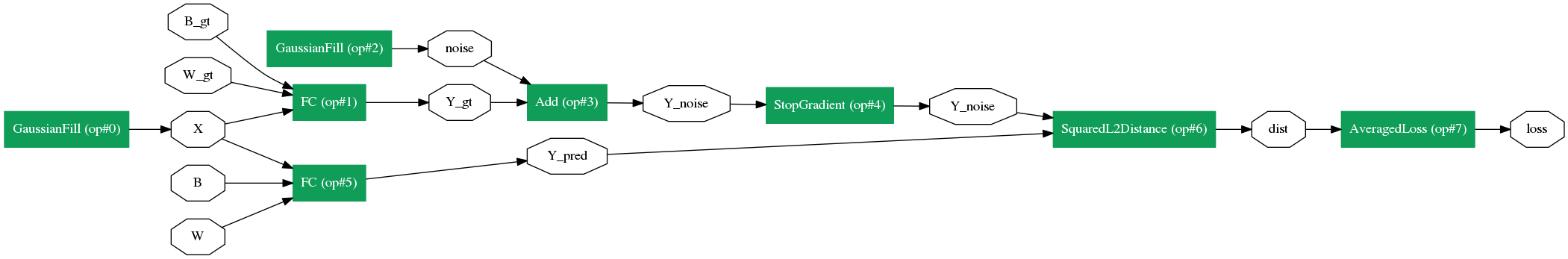
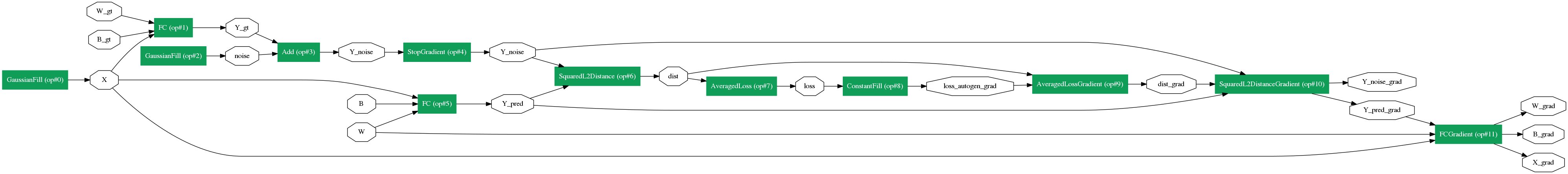
自动生成梯度如上所示意。
SGD部分
#Increment the iteration by one
train_net.Iter(ITER,ITER)
#compute the learning rate that corresponds to the iteration
LR=train_net.LearningRate(ITER,'LR",base_lr=-0.1,policy="step",stepsize=20,gamma=0.9)

# Weighted sum
train_net.WeightedSum([W, ONE, gradient_map[W], LR], W)
train_net.WeightedSum([B, ONE, gradient_map[B], LR], B)

# Let's show the graph again.
graph = net_drawer.GetPydotGraph(train_net.Proto().op, "train", rankdir="LR")
display.Image(graph.create_png(), width=800)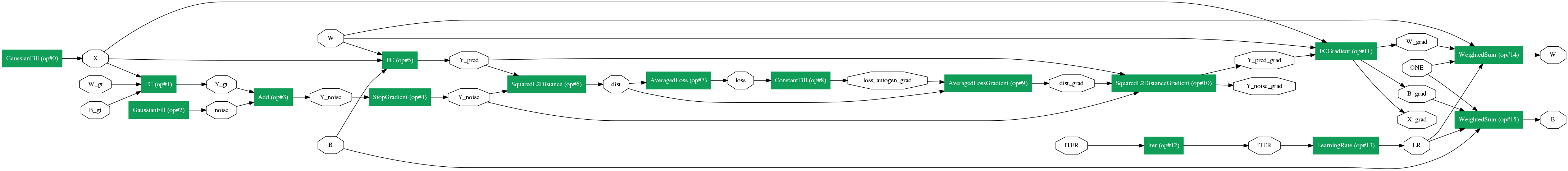
训练网络开始:
workspace.RunNetOnce(init_net)
workspace.CreateNet(train_net)