前言():
{
因为工作的原因,这次更新的比较晚,以后试着跟上进度。
之后大部分的Python学习都是从《神经网络与机器学习第三版》中的习题出发的。
}
正文():
{
本次实验习题比较简单,所以主要收货是对numpy的用法的熟悉。
习题2.8():
{
代码如下:
import numpy as np
#主要函数,其完全按照书上的公式编写
def least_square_for_weight(input_data, input_label, lambda_=0): #①
    data_amount=input_data.shape[0]
    Rxx = [[0,0,0],
          [0,0,0],
          [0,0,0]]
    rdx = [[0],
          [0],
          [0]]
    i = 0
    j = 0
    while i < data_amount:
        while j < data_amount:
            Rxx = Rxx - np.reshape(np.insert(input_data[i],2,1),(3,1)) * np.insert(input_data[j],2,1)
            j = j + 1
        rdx = rdx - np.reshape(np.insert(input_data[i],2,1),(3,1)) * input_label[i]
        i = i + 1
    return np.dot(np.linalg.inv(Rxx+np.identity(3)*lambda_), rdx) #②
#计算并打印决策边界(权值)
print(least_square_for_weight(np.loadtxt("training_sample.txt"), np.loadtxt("training_label.txt",'int'))) ①刚开始我直接用lambda作变量名,发现其已经被Python定义了,其具体用法我参考了:http://blog.csdn.net/lemon_tree12138/article/details/50774827,也因此发现了一种函数的简化形式。
②关于numpy的乘法,参考了http://blog.csdn.net/bbbeoy/article/details/72576863。如果想得到比乘数小的结果,就需要使用点积函数。值得注意的是,使用点积函数需要对齐,比如Rxx的计算就不能用点积函数。
结果如下(lambda_=0):
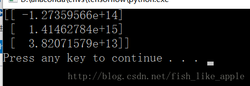
可以看出,决策边界贴近x轴并稍微向逆时针方向偏转。
}
习题2.9():
{
为了大概了解lambda_与决策边界的关系,我用了空间散点图。代码如下:
import numpy as np
#主要函数,其完全按照书上的公式编写
def least_square_for_weight(input_data, input_label, lambda_=0): #①
    data_amount=input_data.shape[0]
    Rxx = [[0,0,0],
          [0,0,0],
          [0,0,0]]
    rdx = [[0],
          [0],
          [0]]
    i = 0
    j = 0
    while i < data_amount:
        while j < data_amount:
            Rxx = Rxx - np.reshape(np.insert(input_data[i],2,1),(3,1)) * np.insert(input_data[j],2,1)
            j = j + 1
        rdx = rdx - np.reshape(np.insert(input_data[i],2,1),(3,1)) * input_label[i]
        i = i + 1
    return np.dot(np.linalg.inv(Rxx+np.identity(3)*lambda_), rdx) #②

def data_displayer_in_3D(X, Y, Z):
    from mpl_toolkits.mplot3d import Axes3D
    import matplotlib.pyplot as plt
    fig = plt.figure()
    ax = fig.add_subplot(111, projection='3d')
    ax.scatter(X, Y, Z, c='r', marker='o')
    plt.show()

#显示决策边界的参数(y=kx+b中的k和b)和lambda_的空间曲线(100个点)
X = np.empty([1,100])
Y = np.empty([1,100])
Z = np.empty([1,100])
i = 0
while i < 100:
    Z[0,i] = (i*0.03)*(i*0.03)*(i*0.03)*(i*0.03)*(i*0.03)*(i*0.03)*(i*0.03)*(i*0.03)*(i*0.03)*(i*0.03)
    XY = least_square_for_weight(np.loadtxt("training_sample.txt"),np.loadtxt("training_label.txt",'int'),Z[0,i])
    X[0,i] = -XY[0,0] / XY[1,0]
    Y[0,i] = -XY[2,0] / XY[1,0]
    if i%10 == 0:
        print(i/10) #显示进度
    i = i + 1
data_displayer_in_3D(X, Y, Z)
结果如下:
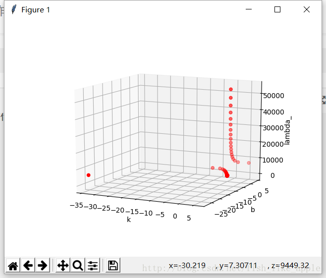
k与lambda_:

b与lambda_:
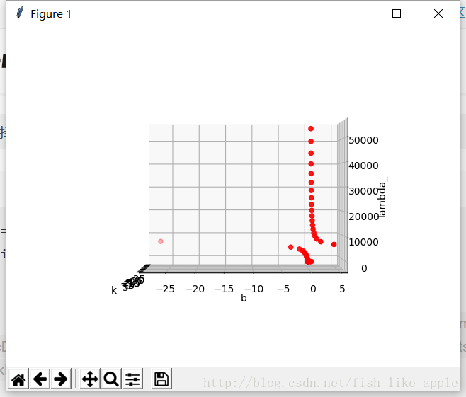
可以看到,当lambda_在7500左右时,决策边界有一次很大的变化;其他情况下,决策边界接近x轴。至于为什么,等到书看一段时间再解决{问题1}。
}
结语():
{
因为我手上的资料没有本章和其他几章的习题答案,所以也没法很快确认是否正确。如果以后我发现错误了,再回来修改。
}