版权声明:本文为博主原创文章,未经博主允许不得转载。 https://blog.csdn.net/u014281392/article/details/83188997
TSAP : TimeSeries Analysis with Python
import pandas as pd
import numpy as np
import matplotlib.pyplot as plt
%matplotlib inline
data = pd.read_csv('data/AirPassengers.csv')
data.head(3)
|
Month |
#Passengers |
| 0 |
1949-01 |
112 |
| 1 |
1949-02 |
118 |
| 2 |
1949-03 |
132 |
data.rename(index=str, columns={'Month':'Date'}, inplace=True)

data['Year'] = data.Date.apply(lambda x: x.split('-')[0])

data['Month'] = data.Date.apply(lambda x: x.split('-')[1])

data.set_index('Date',inplace=True)

data.head(3)
|
#Passengers |
Year |
Month |
| Date |
|
|
|
| 1949-01 |
112 |
1949 |
01 |
| 1949-02 |
118 |
1949 |
02 |
| 1949-03 |
132 |
1949 |
03 |
data['1949-01':'1949-05']
|
#Passengers |
Year |
Month |
| Date |
|
|
|
| 1949-01 |
112 |
1949 |
01 |
| 1949-02 |
118 |
1949 |
02 |
| 1949-03 |
132 |
1949 |
03 |
| 1949-04 |
129 |
1949 |
04 |
| 1949-05 |
121 |
1949 |
05 |
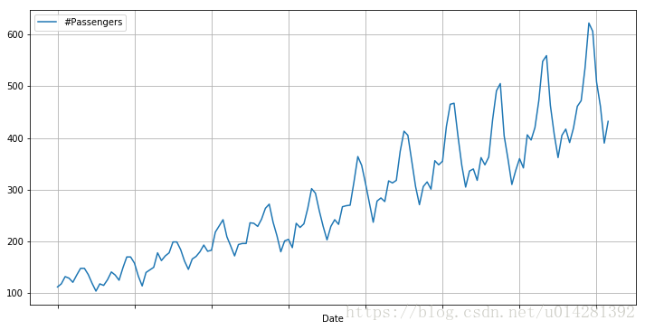
data[['#Passengers']].plot(grid=True, figsize=(12, 6))
dateparse = lambda x, y: pd.datetime.strptime('%s-%s'%(x,y), '%Y-%m')
df = pd.DataFrame({'year': [2015, 2016, 2017, 2018],
'month': [2, 3, 4, 5],
'day': [4, 5, 6, 7],
'hour': [2, 3, 4, 5]})
df
|
day |
hour |
month |
year |
| 0 |
4 |
2 |
2 |
2015 |
| 1 |
5 |
3 |
3 |
2016 |
| 2 |
6 |
4 |
4 |
2017 |
| 3 |
7 |
5 |
5 |
2018 |
pd.to_datetime(df)
0   2015-02-04 02:00:00
1   2016-03-05 03:00:00
2   2017-04-06 04:00:00
3   2018-05-07 05:00:00
dtype: datetime64[ns]
pd.to_datetime(df[['year', 'month', 'day']])
0   2015-02-04
1   2016-03-05
2   2017-04-06
3   2018-05-07
dtype: datetime64[ns]
ts = pd.Series(range(10), index = pd.date_range('8/31/2017', freq = 'M', periods = 10))
ts.truncate(before='10/31/2017', after='5/31/2018')
2017-10-31    2
2017-11-30    3
2017-12-31    4
2018-01-31    5
2018-02-28    6
2018-03-31    7
2018-04-30    8
2018-05-31    9
Freq: M, dtype: int64
ts[[0, 2, 6]].index
DatetimeIndex(['2017-08-31', '2017-10-31', '2018-02-28'], dtype='datetime64[ns]', freq=None)