吴恩达神经网络与深度学习——浅层神经网络习题3
浅层神经网络
实现具有单个隐藏层的两分类神经网络
使用具有非线性激活,如tanh
计算交叉熵损失
实现向前和向后传播
包
numpy
matplotlib
sklearn
# Package imports
import numpy as np
import matplotlib.pyplot as plt
from testCases import *
import sklearn
import sklearn.datasets
import sklearn.linear_model
from planar_utils import plot_decision_boundary, sigmoid, load_planar_dataset, load_extra_datasets

%matplotlib inline

np.random.seed(1) # set a seed so that the results are consistent
数据集
#planar_utils.py
import matplotlib.pyplot as plt
import numpy as np
import sklearn
import sklearn.datasets
import sklearn.linear_model

def plot_decision_boundary(model, X, y):
    # Set min and max values and give it some padding
    x_min, x_max = X[0, :].min() - 1, X[0, :].max() + 1
    y_min, y_max = X[1, :].min() - 1, X[1, :].max() + 1
    h = 0.01
    # Generate a grid of points with distance h between them
    xx, yy = np.meshgrid(np.arange(x_min, x_max, h), np.arange(y_min, y_max, h))
   # np.meshgrid函数将参数1当做第1个结果的每一行, 并且一共有参数2的长度个行。
   	#第2个结果的每一列为参数2的内容, 并且重复参数1的长度个列。
    # Predict the function value for the whole grid
    Z = model(np.c_[xx.ravel(), yy.ravel()])
    #np.ravel将多维数组降为一维,返回的是视图,修改时会影响原始矩阵
    #np.r_是按列连接两个矩阵,就是把两矩阵上下相加,要求列数相等,类似于pandas中的concat()
    #np.c_是按行连接两个矩阵,就是把两矩阵左右相加,要求行数相等,类似于pandas中的merge()。
    Z = Z.reshape(xx.shape)
    # Plot the contour and training examples
    plt.contourf(xx, yy, Z, cmap=plt.cm.Spectral)
    plt.ylabel('x2')
    plt.xlabel('x1')
    plt.scatter(X[0, :], X[1, :], c=y.ravel(), cmap=plt.cm.Spectral)


def sigmoid(x):
    s = 1/(1+np.exp(-x))
    return s

def load_planar_dataset():
    np.random.seed(1)
    m = 400 # number of examples
    N = int(m/2) # number of points per class
    D = 2 # dimensionality
    X = np.zeros((m,D)) # data matrix where each row is a single example
    Y = np.zeros((m,1), dtype='uint8') # labels vector (0 for red, 1 for blue)
    a = 4 # maximum ray of the flower

    for j in range(2):
        ix = range(N*j,N*(j+1))
        t = np.linspace(j*3.12,(j+1)*3.12,N) + np.random.randn(N)*0.2 # theta
        r = a*np.sin(4*t) + np.random.randn(N)*0.2 # radius
        X[ix] = np.c_[r*np.sin(t), r*np.cos(t)]
        Y[ix] = j

    X = X.T
    Y = Y.T

    return X, Y

def load_extra_datasets():
    N = 200
    noisy_circles = sklearn.datasets.make_circles(n_samples=N, factor=.5, noise=.3)
    ## datasets.make_circles()专门用来生成圆圈形状的二维样本.
    #factor表示里圈和外圈的距离之比.每圈共有n_samples/2个点
    # 里圈代表一个类,外圈也代表一个类.noise表示有0.3的点是异常点
    noisy_moons = sklearn.datasets.make_moons(n_samples=N, noise=.2)
    #生成半环形图
    blobs = sklearn.datasets.make_blobs(n_samples=N, random_state=5, n_features=2, centers=6)
    #make_blobs会根据用户指定的特征数量、中心点数量、范围等来生成几类数据,这些数据可用于测试聚类算法的效果。
    #n_samples是待生成的样本的总数。
    #n_features是每个样本的特征数。
    #centers表示类别数。
    #cluster_std表示每个类别的方差,例如我们希望生成2类数据,其中一类比另一类具有更大的方差,可以将cluster_std设置为[1.0,3.0]。
    gaussian_quantiles = sklearn.datasets.make_gaussian_quantiles(mean=None, cov=0.5, n_samples=N, n_features=2, n_classes=2, shuffle=True, random_state=None)
    #利用高斯分位点区分不同数据
    no_structure = np.random.rand(N, 2), np.random.rand(N, 2)

    return noisy_circles, noisy_moons, blobs, gaussian_quantiles, no_structure
import numpy as np

def layer_sizes_test_case():
    np.random.seed(1)
    X_assess = np.random.randn(5, 3)
    Y_assess = np.random.randn(2, 3)
    return X_assess, Y_assess

def initialize_parameters_test_case():
    n_x, n_h, n_y = 2, 4, 1
    return n_x, n_h, n_y

def forward_propagation_test_case():
    np.random.seed(1)
    X_assess = np.random.randn(2, 3)

    parameters = {'W1': np.array([[-0.00416758, -0.00056267],
        [-0.02136196,  0.01640271],
        [-0.01793436, -0.00841747],
        [ 0.00502881, -0.01245288]]),
     'W2': np.array([[-0.01057952, -0.00909008,  0.00551454,  0.02292208]]),
     'b1': np.array([[ 0.],
        [ 0.],
        [ 0.],
        [ 0.]]),
     'b2': np.array([[ 0.]])}

    return X_assess, parameters

def compute_cost_test_case():
    np.random.seed(1)
    Y_assess = np.random.randn(1, 3)
    parameters = {'W1': np.array([[-0.00416758, -0.00056267],
        [-0.02136196,  0.01640271],
        [-0.01793436, -0.00841747],
        [ 0.00502881, -0.01245288]]),
     'W2': np.array([[-0.01057952, -0.00909008,  0.00551454,  0.02292208]]),
     'b1': np.array([[ 0.],
        [ 0.],
        [ 0.],
        [ 0.]]),
     'b2': np.array([[ 0.]])}

    a2 = (np.array([[ 0.5002307 ,  0.49985831,  0.50023963]]))

    return a2, Y_assess, parameters

def backward_propagation_test_case():
    np.random.seed(1)
    X_assess = np.random.randn(2, 3)
    Y_assess = np.random.randn(1, 3)
    parameters = {'W1': np.array([[-0.00416758, -0.00056267],
        [-0.02136196,  0.01640271],
        [-0.01793436, -0.00841747],
        [ 0.00502881, -0.01245288]]),
     'W2': np.array([[-0.01057952, -0.00909008,  0.00551454,  0.02292208]]),
     'b1': np.array([[ 0.],
        [ 0.],
        [ 0.],
        [ 0.]]),
     'b2': np.array([[ 0.]])}

    cache = {'A1': np.array([[-0.00616578,  0.0020626 ,  0.00349619],
         [-0.05225116,  0.02725659, -0.02646251],
         [-0.02009721,  0.0036869 ,  0.02883756],
         [ 0.02152675, -0.01385234,  0.02599885]]),
  'A2': np.array([[ 0.5002307 ,  0.49985831,  0.50023963]]),
  'Z1': np.array([[-0.00616586,  0.0020626 ,  0.0034962 ],
         [-0.05229879,  0.02726335, -0.02646869],
         [-0.02009991,  0.00368692,  0.02884556],
         [ 0.02153007, -0.01385322,  0.02600471]]),
  'Z2': np.array([[ 0.00092281, -0.00056678,  0.00095853]])}
    return parameters, cache, X_assess, Y_assess

def update_parameters_test_case():
    parameters = {'W1': np.array([[-0.00615039,  0.0169021 ],
        [-0.02311792,  0.03137121],
        [-0.0169217 , -0.01752545],
        [ 0.00935436, -0.05018221]]),
 'W2': np.array([[-0.0104319 , -0.04019007,  0.01607211,  0.04440255]]),
 'b1': np.array([[ -8.97523455e-07],
        [  8.15562092e-06],
        [  6.04810633e-07],
        [ -2.54560700e-06]]),
 'b2': np.array([[  9.14954378e-05]])}

    grads = {'dW1': np.array([[ 0.00023322, -0.00205423],
        [ 0.00082222, -0.00700776],
        [-0.00031831,  0.0028636 ],
        [-0.00092857,  0.00809933]]),
 'dW2': np.array([[ -1.75740039e-05,   3.70231337e-03,  -1.25683095e-03,
          -2.55715317e-03]]),
 'db1': np.array([[  1.05570087e-07],
        [ -3.81814487e-06],
        [ -1.90155145e-07],
        [  5.46467802e-07]]),
 'db2': np.array([[ -1.08923140e-05]])}
    return parameters, grads

def nn_model_test_case():
    np.random.seed(1)
    X_assess = np.random.randn(2, 3)
    Y_assess = np.random.randn(1, 3)
    return X_assess, Y_assess

def predict_test_case():
    np.random.seed(1)
    X_assess = np.random.randn(2, 3)
    parameters = {'W1': np.array([[-0.00615039,  0.0169021 ],
        [-0.02311792,  0.03137121],
        [-0.0169217 , -0.01752545],
        [ 0.00935436, -0.05018221]]),
     'W2': np.array([[-0.0104319 , -0.04019007,  0.01607211,  0.04440255]]),
     'b1': np.array([[ -8.97523455e-07],
        [  8.15562092e-06],
        [  6.04810633e-07],
        [ -2.54560700e-06]]),
     'b2': np.array([[  9.14954378e-05]])}
    return parameters, X_assess
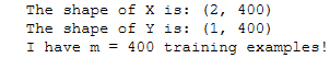
X和Y的尺寸
X, Y = load_planar_dataset()
### START CODE HERE ### (≈ 3 lines of code)
shape_X = X.shape
shape_Y = Y.shape
m =  Y.size # training set size
### END CODE HERE ###

print ('The shape of X is: ' + str(shape_X))
print ('The shape of Y is: ' + str(shape_Y))
print ('I have m = %d training examples!' % (m))
可视化
使用matplotlib可视化数据集。数据看起来像一朵“花”,有一些红色(标记为y = 0 )和一些蓝色( y = 1 )点。你的目标是建立一个模型来拟合这些数据。
plt.scatter(X[0, :], X[1, :], c=Y[0, :], s=40, cmap=plt.cm.Spectral);

逻辑回归
# Train the logistic regression classifier
clf = sklearn.linear_model.LogisticRegressionCV(cv=5);
clf.fit(X.T, Y.T.ravel());
# Plot the decision boundary for logistic regression
plot_decision_boundary(lambda x: clf.predict(x), X, Y)
plt.title("Logistic Regression")

# Print accuracy
LR_predictions = clf.predict(X.T)
print ('Accuracy of logistic regression: %d ' % float((np.dot(Y,LR_predictions) + np.dot(1-Y,1-LR_predictions))/float(Y.size)*100) +
       '% ' + "(percentage of correctly labelled datapoints)")

神经网络
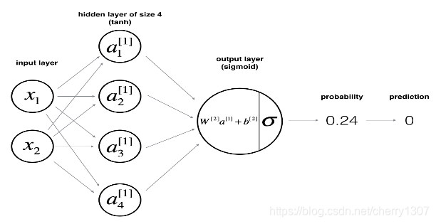

定义神经网络结构
# GRADED FUNCTION: layer_sizes

def layer_sizes(X, Y):
    """
    Arguments:
    X -- input dataset of shape (input size, number of examples)
    Y -- labels of shape (output size, number of examples)

    Returns:
    n_x -- the size of the input layer
    n_h -- the size of the hidden layer
    n_y -- the size of the output layer
    """
    ### START CODE HERE ### (≈ 3 lines of code)
    n_x = X.shape[0] # size of input layer
    n_h = 4
    n_y = Y.shape[0] # size of output layer
    ### END CODE HERE ###
    return (n_x, n_h, n_y)
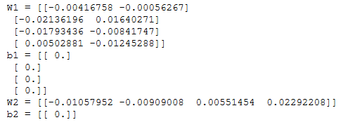
初始化参数
# GRADED FUNCTION: initialize_parameters

def initialize_parameters(n_x, n_h, n_y):
    """
    Argument:
    n_x -- size of the input layer
    n_h -- size of the hidden layer
    n_y -- size of the output layer

    Returns:
    params -- python dictionary containing your parameters:
                    W1 -- weight matrix of shape (n_h, n_x)
                    b1 -- bias vector of shape (n_h, 1)
                    W2 -- weight matrix of shape (n_y, n_h)
                    b2 -- bias vector of shape (n_y, 1)
    """

    np.random.seed(2) # we set up a seed so that your output matches ours although the initialization is random.

    ### START CODE HERE ### (≈ 4 lines of code)
    W1 = np.random.randn(n_h, n_x) * 0.01
    b1 = np.zeros((n_h, 1))
    W2 = np.random.randn(n_y, n_h) * 0.01
    b2 = np.zeros((n_y, 1))
    ### END CODE HERE ###

    assert (W1.shape == (n_h, n_x))
    assert (b1.shape == (n_h, 1))
    assert (W2.shape == (n_y, n_h))
    assert (b2.shape == (n_y, 1))

    parameters = {"W1": W1,
                  "b1": b1,
                  "W2": W2,
                  "b2": b2}

    return parameters
n_x, n_h, n_y = initialize_parameters_test_case()

parameters = initialize_parameters(n_x, n_h, n_y)
print("W1 = " + str(parameters["W1"]))
print("b1 = " + str(parameters["b1"]))
print("W2 = " + str(parameters["W2"]))
print("b2 = " + str(parameters["b2"]))
前向传播
# GRADED FUNCTION: forward_propagation

def forward_propagation(X, parameters):
    """
    Argument:
    X -- input data of size (n_x, m)
    parameters -- python dictionary containing your parameters (output of initialization function)

    Returns:
    A2 -- The sigmoid output of the second activation
    cache -- a dictionary containing "Z1", "A1", "Z2" and "A2"
    """
    # Retrieve each parameter from the dictionary "parameters"
    ### START CODE HERE ### (≈ 4 lines of code)
    W1 = parameters["W1"]
    b1 = parameters["b1"]
    W2 = parameters["W2"]
    b2 = parameters["b2"]
    #print(W1.shape, b1.shape, W2.shape, b2.shape)

    ### END CODE HERE ###

    # Implement Forward Propagation to calculate A2 (probabilities)
    ### START CODE HERE ### (≈ 4 lines of code)
    Z1 = np.dot(W1, X) + b1
    A1 = np.tanh(Z1)
    Z2 = np.dot(W2, A1) + b2
    A2 = sigmoid(Z2)
    ### END CODE HERE ###

    assert(A2.shape == (1, X.shape[1]))

    cache = {"Z1": Z1,
             "A1": A1,
             "Z2": Z2,
             "A2": A2}

    return A2, cache
X_assess, parameters = forward_propagation_test_case()

A2, cache = forward_propagation(X_assess, parameters)

# Note: we use the mean here just to make sure that your output matches ours.
print(np.mean(cache['Z1']) ,np.mean(cache['A1']),np.mean(cache['Z2']),np.mean(cache['A2']))

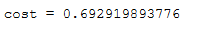
代价函数

# GRADED FUNCTION: compute_cost

def compute_cost(A2, Y, parameters):
    """
    Computes the cross-entropy cost given in equation (13)

    Arguments:
    A2 -- The sigmoid output of the second activation, of shape (1, number of examples)
    Y -- "true" labels vector of shape (1, number of examples)
    parameters -- python dictionary containing your parameters W1, b1, W2 and b2

    Returns:
    cost -- cross-entropy cost given equation (13)
    """

    m = Y.shape[1] # number of example

    # Retrieve W1 and W2 from parameters
    ### START CODE HERE ### (≈ 2 lines of code)
    W1 = parameters["W1"]
    W2 = parameters["W2"]
    ### END CODE HERE ###

    # Compute the cross-entropy cost
    ### START CODE HERE ### (≈ 2 lines of code)
    logprobs = np.multiply(np.log(A2), Y) + np.multiply((1-Y), np.log(1-A2))
    ### END CODE HERE ###
    cost = -1/m * np.sum(logprobs)

    cost = np.squeeze(cost)     # makes sure cost is the dimension we expect.
                                # E.g., turns [[17]] into 17
    assert(isinstance(cost, float))

    return cost
A2, Y_assess, parameters = compute_cost_test_case()

print("cost = " + str(compute_cost(A2, Y_assess, parameters)))
反向传播

# GRADED FUNCTION: backward_propagation

def backward_propagation(parameters, cache, X, Y):
    """
    Implement the backward propagation using the instructions above.

    Arguments:
    parameters -- python dictionary containing our parameters
    cache -- a dictionary containing "Z1", "A1", "Z2" and "A2".
    X -- input data of shape (2, number of examples)
    Y -- "true" labels vector of shape (1, number of examples)

    Returns:
    grads -- python dictionary containing your gradients with respect to different parameters
    """
    m = X.shape[1]

    # First, retrieve W1 and W2 from the dictionary "parameters".
    ### START CODE HERE ### (≈ 2 lines of code)
    W1 = parameters["W1"]
    W2 = parameters["W2"]
    ### END CODE HERE ###

    # Retrieve also A1 and A2 from dictionary "cache".
    ### START CODE HERE ### (≈ 2 lines of code)
    A1 = cache["A1"]
    A2 = cache["A2"]
    ### END CODE HERE ###

    # Backward propagation: calculate dW1, db1, dW2, db2.
    ### START CODE HERE ### (≈ 6 lines of code, corresponding to 6 equations on slide above)
    dZ2= A2 - Y
    dW2 = (1/m) * np.dot(dZ2, A1.T)
    db2 = (1/m) * np.sum(dZ2, axis=1, keepdims=True)
    dZ1 = np.multiply(np.dot(W2.T, dZ2), (1 - np.power(A1, 2)))
    dW1 = (1/m) * np.dot(dZ1, X.T)
    db1 = (1/m) * np.sum(dZ1, axis=1, keepdims=True)
    ### END CODE HERE ###

    grads = {"dW1": dW1,
             "db1": db1,
             "dW2": dW2,
             "db2": db2}

    return grads
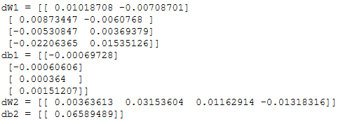
parameters, cache, X_assess, Y_assess = backward_propagation_test_case()

grads = backward_propagation(parameters, cache, X_assess, Y_assess)
print ("dW1 = "+ str(grads["dW1"]))
print ("db1 = "+ str(grads["db1"]))
print ("dW2 = "+ str(grads["dW2"]))
print ("db2 = "+ str(grads["db2"]))
梯度下降

# GRADED FUNCTION: update_parameters

def update_parameters(parameters, grads, learning_rate = 1.2):
    """
    Updates parameters using the gradient descent update rule given above

    Arguments:
    parameters -- python dictionary containing your parameters
    grads -- python dictionary containing your gradients

    Returns:
    parameters -- python dictionary containing your updated parameters
    """
    # Retrieve each parameter from the dictionary "parameters"
    ### START CODE HERE ### (≈ 4 lines of code)
    W1 = parameters["W1"]
    b1 = parameters["b1"]
    W2 = parameters["W2"]
    b2 = parameters["b2"]
    ### END CODE HERE ###

    # Retrieve each gradient from the dictionary "grads"
    ### START CODE HERE ### (≈ 4 lines of code)
    dW1 = grads["dW1"]
    db1 = grads["db1"]
    dW2 = grads["dW2"]
    db2 = grads["db2"]
    ## END CODE HERE ###

    # Update rule for each parameter
    ### START CODE HERE ### (≈ 4 lines of code)
    W1 = W1 - learning_rate * dW1
    b1 = b1 - learning_rate * db1
    W2 = W2 - learning_rate * dW2
    b2 = b2 - learning_rate * db2
    ### END CODE HERE ###

    parameters = {"W1": W1,
                  "b1": b1,
                  "W2": W2,
                  "b2": b2}

    return parameters
parameters, grads = update_parameters_test_case()
parameters = update_parameters(parameters, grads)

print("W1 = " + str(parameters["W1"]))
print("b1 = " + str(parameters["b1"]))
print("W2 = " + str(parameters["W2"]))
print("b2 = " + str(parameters["b2"]))
model
# GRADED FUNCTION: nn_model

def nn_model(X, Y, n_h, num_iterations = 10000, print_cost=False):
    """
    Arguments:
    X -- dataset of shape (2, number of examples)
    Y -- labels of shape (1, number of examples)
    n_h -- size of the hidden layer
    num_iterations -- Number of iterations in gradient descent loop
    print_cost -- if True, print the cost every 1000 iterations

    Returns:
    parameters -- parameters learnt by the model. They can then be used to predict.
    """

    np.random.seed(3)
    n_x = layer_sizes(X, Y)[0]
    n_y = layer_sizes(X, Y)[2]

    # Initialize parameters, then retrieve W1, b1, W2, b2. Inputs: "n_x, n_h, n_y". Outputs = "W1, b1, W2, b2, parameters".
    ### START CODE HERE ### (≈ 5 lines of code)
    parameters = initialize_parameters(n_x, n_h, n_y)
    W1 = parameters["W1"]
    b1 = parameters["b1"]
    W2 = parameters["W2"]
    b2 = parameters["b2"]
    ### END CODE HERE ###

    # Loop (gradient descent)

    for i in range(0, num_iterations):

        ### START CODE HERE ### (≈ 4 lines of code)
        # Forward propagation. Inputs: "X, parameters". Outputs: "A2, cache".
        A2, cache = forward_propagation(X, parameters)

        # Cost function. Inputs: "A2, Y, parameters". Outputs: "cost".
        cost = compute_cost(A2, Y, parameters)

        # Backpropagation. Inputs: "parameters, cache, X, Y". Outputs: "grads".
        grads = backward_propagation(parameters, cache, X, Y)

        # Gradient descent parameter update. Inputs: "parameters, grads". Outputs: "parameters".
        parameters = update_parameters(parameters, grads)

        ### END CODE HERE ###

        # Print the cost every 1000 iterations
        if print_cost and i % 1000 == 0:
            print ("Cost after iteration %i: %f" %(i, cost))

    return parameters
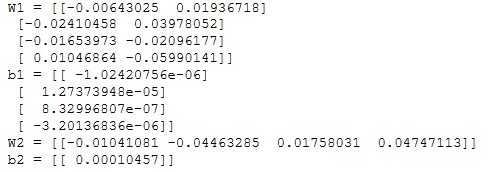
X_assess, Y_assess = nn_model_test_case()

parameters = nn_model(X_assess, Y_assess, 4, num_iterations=10000, print_cost=False)
print("W1 = " + str(parameters["W1"]))
print("b1 = " + str(parameters["b1"]))
print("W2 = " + str(parameters["W2"]))
print("b2 = " + str(parameters["b2"]))

预测

# GRADED FUNCTION: predict

def predict(parameters, X):
    """
    Using the learned parameters, predicts a class for each example in X

    Arguments:
    parameters -- python dictionary containing your parameters
    X -- input data of size (n_x, m)

    Returns
    predictions -- vector of predictions of our model (red: 0 / blue: 1)
    """

    # Computes probabilities using forward propagation, and classifies to 0/1 using 0.5 as the threshold.
    ### START CODE HERE ### (≈ 2 lines of code)
    A2, cache = forward_propagation(X, parameters)
    predictions = (A2 > 0.5)  # Vectorized
    ### END CODE HERE ###

    return predictions
parameters, X_assess = predict_test_case()

predictions = predict(parameters, X_assess)
print("predictions mean = " + str(np.mean(predictions)))

测试
# Build a model with a n_h-dimensional hidden layer
parameters = nn_model(X, Y, n_h = 4, num_iterations = 10000, print_cost=True)

# Plot the decision boundary
plot_decision_boundary(lambda x: predict(parameters, x.T), X, Y)
plt.title("Decision Boundary for hidden layer size " + str(4))
# Print accuracy
predictions = predict(parameters, X)
print ('Accuracy: %d' % float((np.dot(Y,predictions.T) + np.dot(1-Y,1-predictions.T))/float(Y.size)*100) + '%')

调整隐藏层大小
# This may take about 2 minutes to run

plt.figure(figsize=(16, 32))
hidden_layer_sizes = [1, 2, 3, 4, 5, 20, 50]
for i, n_h in enumerate(hidden_layer_sizes):
    plt.subplot(5, 2, i+1)
    plt.title('Hidden Layer of size %d' % n_h)
    parameters = nn_model(X, Y, n_h, num_iterations = 5000)
    plot_decision_boundary(lambda x: predict(parameters, x.T), X, Y)
    predictions = predict(parameters, X)
    accuracy = float((np.dot(Y,predictions.T) + np.dot(1-Y,1-predictions.T))/float(Y.size)*100)
    print ("Accuracy for {} hidden units: {} %".format(n_h, accuracy))
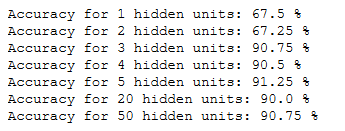
较大的模型(具有更多隐藏单元)能够更好地适应训练集,直到过拟合。
最佳隐藏层尺寸似乎在n _ h = 5左右。事实上,这里的一个值似乎很适合数据,而不会引起明显的过度拟合。
其他数据集的性能
# Datasets
noisy_circles, noisy_moons, blobs, gaussian_quantiles, no_structure = load_extra_datasets()

datasets = {"noisy_circles": noisy_circles,
            "noisy_moons": noisy_moons,
            "blobs": blobs,
            "gaussian_quantiles": gaussian_quantiles}

### START CODE HERE ### (choose your dataset)
dataset = "noisy_moons"
### END CODE HERE ###

X, Y = datasets[dataset]
X, Y = X.T, Y.reshape(1, Y.shape[0])

# make blobs binary
if dataset == "blobs":
    Y = Y%2

# Visualize the data
plt.scatter(X[0, :], X[1, :], c=Y.ravel(), s=40, cmap=plt.cm.Spectral);

np.meshgrid()
np,c_(),np.r_()
np.ravel()和np.flatten()
plt.scatter()
range
klearn的make_circles和make_moons生成数据
py.sklearn.datasets.make_blobs
make_gaussian_quantiles
make_gaussian_quantiles
plt.cm.Spectral
isinstance() 函数