I am a sophomore from UESTC. This is my first time to write a blog, so it you have any suggestions, please let me know.
One of my professors taught us some technology about image processing and I found it pretty interesting, so I did something in Python in my spare time, so I would like to show something about it.
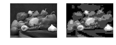
Problem 1: Sampling and Quantization
In this problem, we intend to study the effects of sampling and
quantization on digital images. My job is to write a function with the
following specifications ( may use loops if necessary): (i) The
function takes one input: the image file name, ‘peppers.png’. (ii) The
input image is assumed to be grayscale. (iii) Sample the image in
spatial domain with a sampling rate of 10 (your image should be
approximately 10 times smaller along width and height, do not use any
numpy functions). (iv) Do a 5-level uniform quantization of the
sampled image so that the bins cover the whole range of grayscale
values (0 to 255). You should not use any numpy functions for this.
(v) The function returns one output: the sampled and quantized image.
Below is my code:
  import numpy as np
    from scipy.misc import imread, imresize
    import matplotlib.pyplot as plt

def sampling_quantization(img):
    sampled_image = imresize(img, 0.1)
    img_height = sampled_image.shape[0]
    img_width = sampled_image.shape[1]
    for row in range(img_height):
        for col in range(img_width):
            if sampled_image[row, col] <= 51:
                sampled_image[row, col] = 25
            if sampled_image[row, col] > 51 and sampled_image[row, col] <= 102:
                sampled_image[row, col] = 76
            if sampled_image[row, col] > 102 and sampled_image[row, col] <= 153:
                sampled_image[row, col] = 127
            if sampled_image[row, col] > 153 and sampled_image[row, col] <= 204:
                sampled_image[row, col] = 178
            if sampled_image[row, col] > 204 and sampled_image[row, col] <= 255:
                sampled_image[row, col] = 229
    sampled_quantized_image = sampled_image
    return sampled_quantized_image

img = imread(r'C:\Users\user\Desktop\CV stuff\Task 2\assignment2\peppers.png')
print(img.shape)
sampled_quantized_image = sampling_quantization(img)
plt.subplot(1, 2, 1)
plt.imshow(img, cmap="gray")
plt.axis('off')
plt.subplot(1, 2, 2)
plt.imshow(sampled_quantized_image, cmap="gray")
plt.axis('off')
plt.show()
Here is the output:
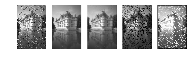
Problem 2: Order-statistic filtering
Order-statistic filters (OSF) are local filters that are only based on
the ranking of pixel values inside a sliding window.Create in imstack(img,s1,s2) function that creates a stack xstack of
size n1 ×n2 ×s, which s = (2s1 +1)(2s2 +1) from the n1 ×n2 image x,
such that xstack(i,j,:) contains all the values of x in the
neighborhood (−s1, s1) × (−s2, s2). This function should take into
account the four possible boundary conditions. (Hint: we can use
imshift, which we implemented in assignment 1, and only two loops for
−s1 <= k <= s1 and −s2<= l<= s2.) Create in imosf() function function
imosf(x, type, s1, s2) that implements order-statistic filters,
returns xosf. imosf should first call imstack, next sort the entries
of the stack with respect to the third dimension, and create the
suitable output xosf according to the string type as follows: •
‘median’: select the median value, • ‘erode’: select the min value, •
‘dilate’: select the max value, • ‘trimmed’: take the mean after
excluding at least 25% of the extreme values on each side. Create in
imopening() and imclosing() function that performs the opening and
closing by the means of OSF filters.
Below is my code:
import numpy as np
from scipy.misc import imread
import matplotlib.pyplot as plt

def noise(img, perc):
    (n1, n2) = img.shape
    salt_ammount = np.ceil(n1*n2*(perc/100)/2)
    pepper_amount = np.ceil(n1*n2*(perc/100)/2)
    noisy_image = img.copy()
    for i in range(int(salt_ammount)):
        x = np.random.randint(0, n1)
        y = np.random.randint(0, n2)
        noisy_image[x, y] = 255
    for j in range(int(pepper_amount)):
        x = np.random.randint(0, n1)
        y = np.random.randint(0, n2)
        noisy_image[x, y] = 0
    return noisy_image

def imstack(img,s1,s2):
    (n1, n2) = img.shape
    s = (2*s1 + 1) * (2*s2 + 1)
    xstack = np.zeros((n1, n2, s))
    for i in range(s1, n1 - s1):
        for j in range(s2, n2 - s2):
            image_block = img[i - s1:i + s1 + 1, j - s2:j + s2 + 1]
            for a in range(2 * s1 + 1):
                for b in range(2 * s2 + 1):
                    xstack[i, j, (2 * s1 + 1) * a + b] = image_block[a, b]

    return xstack

def imosf(img, typ, s1, s2):
    (n1, n2) = img.shape
    imosf_image = np.zeros((n1, n2))
    xstack = imstack(img, s1, s2)
    for row in range(n1):
            for col in range(n2):
                if typ == 'dialate':
                    imosf_image[row, col] = np.max(xstack[row, col, :])

                if typ == 'erode':
                    imosf_image[row, col] = np.min(xstack[row, col, :])

                if typ == 'median':
                    sort_array = np.sort(xstack[row, col, :], axis=0)
                    middle_value = sort_array[int(((2 * s1 + 1) * (2 * s2 + 1) - 1) / 2)]
                    imosf_image[row, col] = middle_value

                if typ == 'trimmed':
                    sort_array = np.sort(xstack[row, col, :], axis=0)
                    sort_array = sort_array[int(((2 * s1 + 1)*(2 * s2 + 1)-1)/2/4) : int((2 * s1 + 1)*(2 * s2 + 1)-((2 * s1 + 1)*(2 * s2 + 1)-1)/2/4)]
                    mean_value = np.sum(sort_array)/np.shape(sort_array)[0]
                    imosf_image[row, col] = mean_value


    return imosf_image

def imopening(img, s1, s2):
    imopening_image = imosf(img, 'dialate', s1, s2)
    imopening_image = imosf(imopening_image, 'erode', s1, s2)
    return imopening_image

def imclosing(img, s1, s2):
    imclosing_image = imosf(img, 'erode', s1, s2)
    imclosing_image = imosf(imclosing_image, 'dialate', s1, s2)
    return imclosing_image

img = imread(r'C:\Users\user\Desktop\CV stuff\Task 3\assignment3\castle.png')
s1 = 2
s2 = 2
noisy_image = noise(img, 10)
immedian_image = imosf(noisy_image, 'median', s1, s2)
imtrimmed_image = imosf(noisy_image, 'trimmed', s1, s2)
imopening_image = imopening(noisy_image, s1, s2)
imclosing_image = imclosing(noisy_image, s1, s2)
plt.subplot(1, 5, 1)
plt.imshow(noisy_image, cmap="gray")
plt.axis('off')
plt.subplot(1, 5, 2)
plt.imshow(immedian_image, cmap="gray")
plt.axis('off')
plt.subplot(1, 5, 3)
plt.imshow(imtrimmed_image, cmap="gray")
plt.axis('off')
plt.subplot(1, 5, 4)
plt.imshow(imclosing_image, cmap="gray")
plt.axis('off')
plt.subplot(1, 5, 5)
plt.imshow(imopening_image, cmap="gray")
plt.axis('off')
plt.show()
Here is the output:
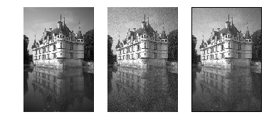
Problem 3: Bilateral filter
Now, we will discuss a non-local filter, Bilateral filter. The
bilateral filter is a denoising algorithm that reads as: Create a
test_imbilateral(img, sigma) function that loads the image x = castle
and adds additive white Gaussian noise of standard deviation σ = 10
Create in imbilateral_naive(img, sigma, s1, s2, h), a function that
implements the bilateral filter (except around boundaries) with four
loops. test your function on y with s1 = s2 = 10 and h = 1. Zoom on
the results to check that your functions are consistent with the
following ones:
Below is my code:
import numpy as np
from scipy.misc import imread
import matplotlib.pyplot as plt
import random

def GaussianNoise(img, means, sigma):
    n1, n2 = img.shape
    noise_img = np.zeros((n1, n2))
    for i in range(n1):
        for j in range(n2):
            noise_img[i, j] = img[i, j] + random.gauss(means, sigma)
            if noise_img[i, j] < 0:
                noise_img[i, j] = 0
            elif noise_img[i, j] > 255:
                noise_img[i, j] = 255

    return noise_img

def imstack(img,s1,s2):
    (n1, n2) = img.shape
    s = (2*s1 + 1) * (2*s2 + 1)
    xstack = np.zeros((n1, n2, s))
    for i in range(s1, n1 - s1):
        for j in range(s2, n2 - s2):
            image_block = img[i - s1:i + s1 + 1, j - s2:j + s2 + 1]
            for a in range(2 * s1 + 1):
                for b in range(2 * s2 + 1):
                    xstack[i, j, (2 * s1 + 1) * a + b] = image_block[a, b]

    return xstack

def imkernel_space(tau, s1, s2):
    w = lambda i, j: np.exp(-(i**2 + j**2)/(2*tau**2))
    i, j = np.mgrid[-s1:s1 + 1, -s2:s2 + 1]
    nu = lambda i, j: w(i, j)

    return nu

def imkernel_value(central_value, amount, tau, s1, s2, xstack, i, j):
    w = lambda i: np.exp(-(i ** 2)/(2*tau**2))
    xstack_segment = np.zeros(amount)
    for t in range(amount):
        xstack_segment[t] = w((central_value-xstack[i, j, t]))
    xstack_segment_anoform = np.zeros((2 * s1 + 1, 2 * s2 + 1))
    for a in range(2 * s1 + 1):
        for b in range(2 * s2 + 1):
            xstack_segment_anoform[a, b] = xstack_segment[a * (2 * s1 + 1) + b]

    return xstack_segment_anoform

def imkernel_mul(xstack_segment_anoform, nu, s1, s2):
    mul_coefficient = np.zeros((2 * s1 + 1, 2 * s2 + 1))
    k = -s1
    for a in range(2 * s1 + 1):
        l = -s2
        for b in range(2 * s2 + 1):
            mul_coefficient[a, b] = xstack_segment_anoform[a, b] * nu(k, l)
            l = l + 1
        k = k + 1
    sum = np.sum(mul_coefficient)
    mul_coefficient = mul_coefficient/sum

    return mul_coefficient

def imbilateral_naive(x, xstack, nu, sigma, s1, s2):
    n1, n2 = np.shape(x)
    xconv = np.zeros((n1, n2))
    m1, m2, m3 = np.shape(xstack)
    for i in range(s1, n1 - s1):
        for j in range(s2, n2 - s2):
            central_value = x[i, j]
            xstack_segment_anoform = imkernel_value(central_value, m3, sigma, s1, s2, xstack, i, j)
            mul_coefficient = imkernel_mul(xstack_segment_anoform, nu, s1, s2)
            k = i
            for a in range(2 * s1 + 1):
                l = j
                for b in range(2 * s2 + 1):
                    xconv[i, j] = xconv[i, j] + mul_coefficient[a, b] * x[k - s1, l - s2]
                    l = l + 1
                k = k + 1
    return xconv

img = imread(r'C:\Users\user\Desktop\CV stuff\Task 3\assignment3\castle.png')
means = 0
sigma = 10
gaussnoise_img = GaussianNoise(img, means, sigma)
sigma_space = 10
sigma_value = 10
s1 = 2
s2 = 2
nu = imkernel_space(sigma_space, s1, s2)
xstack = imstack(gaussnoise_img, s1, s2)
img_processed = imbilateral_naive(gaussnoise_img, xstack, nu, sigma_value, s1, s2)
plt.subplot(1, 3, 1)
plt.imshow(img, cmap="gray")
plt.axis('off')
plt.subplot(1, 3, 2)
plt.imshow(gaussnoise_img, cmap="gray")
plt.axis('off')
plt.subplot(1, 3, 3)
plt.imshow(img_processed, cmap="gray")
plt.axis('off')
plt.show()
Here is the output:
Thank you for reading this!