::::::::线性回归::::::::
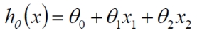 第一式
第一式
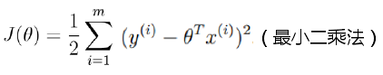
 第二式
第二式
从式一到式二,需要添加一个 项,其中
为
= 1 的常数量。只是为了容易写成代码而已。

真实值=预测值+误差(误差是独立且具有相同的分布,通常认为服从均值为0的方差为 的高斯分布。)

![]() 此式意思是要找到一个θ值使得该θ与x的组合完之后,使得组合值接近y真实值的概率最大化。
此式意思是要找到一个θ值使得该θ与x的组合完之后,使得组合值接近y真实值的概率最大化。
为了使得概率最大,我们用到了似然函数。

我们所希望的到的L(θ)的值是越大越好——代表了所有的y(i)与其真实值都是尽可能相等的。击球什么样的θ可以使得L(θ)的整体值是最大的。
- 为了使得求解变得简单一些,我们引入对数似然函数 l(θ) = ln L(θ)


- 牢记,咱们要求的是似然函数L(θ)的值尽可能大,也就是使对数似然函数l(θ)的最大值,通过化简的到上式,所以咱们要做的就是使右式J(θ)值最小。!
- 关于J(θ)的求解:

(上面第二步是对 θ 求偏导操作,矩阵求导不做解释,不过可以从上图看出一二)
#以下代码是对以上原理的简单应用。目前我的环境尚未搭建妥当,所以还没有去跑代码,先码在这里,等之后参考

import matplotlib.pyplot as plt
import numpy as np
from sklearn import datasets

class LinearRegression():
    def __init__(self):
        self.w = None
    def fit(self,X,y):
        #训练阶段
        #Insert constant ones for bias weights
        print (X.shape)
        #x0 = 1
        X=np.insert(X,0,1,axis=1)
        print (X.shape)
        #对X的转置取逆操作。
        X_ = np.linalg.iniv(X.T.dot(X))
        self.w = X_.dot(X.T).dot(y)
    def predict(self,X):
        #测试阶段
        #Insert constant ones for bias weights
        X = np.insert(X,0,1,axis=1)
        y_pred = X.dot(self.w)
        return y_pred

def mean_squared_error(y_true, ypred):
    mse = np.mean(np.power(y_true - y_pred, 2))
    return mse


def main():
    #Load the diabetes dataset
    diabetes = datasets.load_diabetes()

    #Use only one feature
    X = diabetes.data[:, np.newaxis, 2]
    print(X.shape)

    #Split the data into training/testing sets
    x_train, x_test = X[:-20],X[-20:]

    #Split the targets into training/testing sets
    y_train, y_test = diabetes.target[:-20], diabetes.target[-20:]

    clf = LinearRegression()
    clf.fit(x_train, y_train)
    y_pred = clf.predict(x_test)

    #Print the mean squared error
    print ("Mean Souared Error:"mean_squared_error(y_test, y_pred))

    #Plot the results
    plt.scatter(x_test[:,0], y_test, color='black')
    plt.plot(x_test[:,0], y_pred, color='blue',linewidth=3)
    plt.show()
参考:
机器学习课程——唐老师