版权声明:本文为博主原创文章,未经博主允许不得转载。 https://blog.csdn.net/LRH2018/article/details/80465818
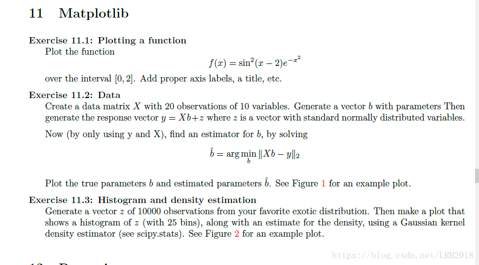
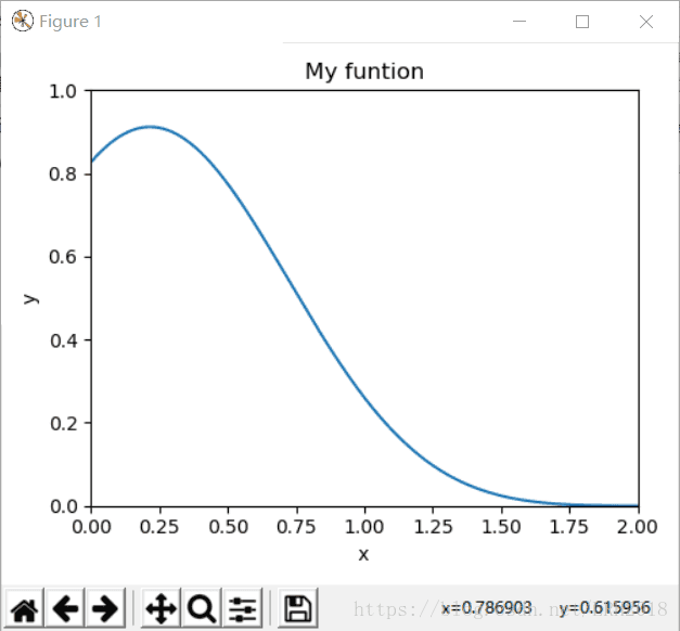
Exercise 11.1
import numpy as np
import matplotlib.pyplot as plt
import seaborn as sns
import math

f, ax = plt.subplots(1, 1, figsize=(5,4))
x = np.linspace(0, 2, 1000)                                #取点
y = [pow(math.sin(z-2), 2)* pow(math.e, -z*z) for z in x]  #函数方程求对应函数值

ax.plot(x, y)
ax.set_xlim((0, 2))
ax.set_ylim((0, 1))
ax.set_xlabel(' x ')
ax.set_ylabel(' y ')
ax.set_title('My funtion')

plt.tight_layout()
plt.show()

#plt.savefig('line_plot_plus.png') #保存为图片
绘制图像如图:
Exercise 11.2
import numpy as np
import matplotlib.pyplot as plt
import seaborn as sns
import math

x = np.random.rand(20, 10)

b = np.random.rand(10, 1)

z = np.random.normal(loc = 0, scale = 1, size = (20, 1))

x = np.mat(x)
b = np.mat(b)
z = np.mat(z)

y = x * b + z
s = x.T * x
s = s.I * x.T
b_ = s * y

b_ = np.array(b_)
b  = np.array(b)

X = np.arange(0, 10)
plt.title('Parameter plot')
plt.xlabel('index')
plt.ylabel('value')
plt.scatter(X, b, c='r', marker='o', label='b')
plt.scatter(X, b_, c='b', marker='x', label='b^')
plt.legend()
plt.show ()
plt.tight_layout()
plt.show()
运行结果

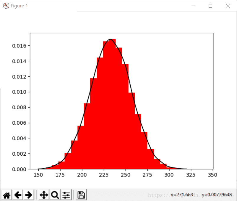
Exercise 11.3
import numpy as np
import matplotlib.pyplot as plt
import seaborn as sns
import math
import scipy.stats

z = np.random.normal(loc=233, scale=23.3, size=10000)

plt.hist(z , bins=25, density = True, color='r')

kernel = scipy.stats.gaussian_kde(z)

x = np.linspace(150, 320, 10000)
plt.plot(x, kernel(x), 'k' )

plt.show()