本文原是xgboost的官方文档教程,但是鉴于其中部分内容叙述不清,部分内容也确实存在一定的问题,所以本人重写了该部分。数据请前往Github此处下载
前置代码
引用类库,添加需要的函数
import numpy as np
from sklearn.model_selection import train_test_split
import xgboost as xgb
import pandas as pd
import matplotlib
%matplotlib inline
def GetNewDataByPandas():
    wine = pd.read_csv("/Data/UCI/wine/wine.csv")
    wine['alcohol**2'] = pow(wine["alcohol"], 2)
    wine['volatileAcidity*alcohol'] = wine["alcohol"] * wine['volatile acidity']
    y = np.array(wine.quality)
    X = np.array(wine.drop("quality", axis=1))
    # X = np.array(wine)

    columns = np.array(wine.columns)

    return X, y, columns
直接从csv加载亦可
file_path = "/home/fonttian/Data/UCI/wine/wine.csv"
data = np.genfromtxt(file_path, delimiter=',')
dtrain_2 = xgb.DMatrix(data[1:1119, 0:11], data[1:1119, 11])
dtest_2 = xgb.DMatrix(data[1119:1599, 0:11], data[1119:1599, 11])
加载数据
读取数据并分割
# Read wine quality data from file
X, y, wineNames = GetNewDataByPandas()
# X, y, wineNames = GetDataByPandas()
# split data to [0.8,0.2,01]
x_train, x_predict, y_train, y_predict = train_test_split(X, y, test_size=0.10, random_state=100)


# take fixed holdout set 30% of data rows
x_train, x_test, y_train, y_test = train_test_split(x_train, y_train, test_size=0.2, random_state=100)
展示数据
wineNames
array(['fixed acidity', 'volatile acidity', 'citric acid',
       'residual sugar', 'chlorides', 'free sulfur dioxide',
       'total sulfur dioxide', 'density', 'pH', 'sulphates', 'alcohol',
       'quality', 'alcohol**2', 'volatileAcidity*alcohol'], dtype=object)
print(len(x_train),len(y_train))
print(len(x_test))
print(len(x_predict))
1151 1151
288
160
加载到DMatrix
- 其中missing将作为填充缺失数值的默认值,可不填
- 必要时也可以设置权重
dtrain = xgb.DMatrix(data=x_train,label=y_train,missing=-999.0)
dtest = xgb.DMatrix(data=x_test,label=y_test,missing=-999.0)

# w = np.random.rand(5, 1)
# dtrain = xgb.DMatrix(x_train, label=y_train, missing=-999.0, weight=w)
设定参数
Booster参数
param = {'max_depth': 7, 'eta': 1, 'silent': 1, 'objective': 'reg:linear'}
param['nthread'] = 4
param['seed'] = 100
param['eval_metric'] = 'auc'
还可以指定多个ecal指标
param['eval_metric'] = ['auc', 'ams@0']
# 此处我们进行回归运算,只设置rmse
param['eval_metric'] = ['rmse']
param['eval_metric']
['rmse']
指定设置为监视性能的验证
evallist = [(dtest, 'eval'), (dtrain, 'train')]
训练
训练模型
在之前的代码中,我将数据分割为 6:3:1,其分别为,训练数据,性能监视用数据,和最后的预测数据。这个比例只是为了示例用,并不具有代表性。
在数据集不足的情况下,除预测数据外,也可以不分割训练集与验证集,使用交叉验证方法,不适用性能监视数据(验证集)有时也是可行的。请自行思考,进行选择。
num_round = 10
bst_without_evallist = xgb.train(param, dtrain, num_round)
num_round = 10
bst_with_evallist = xgb.train(param, dtrain, num_round, evallist)
[0]	eval-rmse:0.793859	train-rmse:0.68806
[1]	eval-rmse:0.796485	train-rmse:0.474253
[2]	eval-rmse:0.796662	train-rmse:0.450195
[3]	eval-rmse:0.778571	train-rmse:0.400886
[4]	eval-rmse:0.789566	train-rmse:0.340342
[5]	eval-rmse:0.798235	train-rmse:0.27816
[6]	eval-rmse:0.804898	train-rmse:0.244093
[7]	eval-rmse:0.813786	train-rmse:0.212835
[8]	eval-rmse:0.81194	train-rmse:0.190969
[9]	eval-rmse:0.814219	train-rmse:0.159447
模型持久化
models_path = "/home/fonttian/Models/Sklearn_book/xgboost/"
bst_with_evallist.save_model(models_path+'bst_with_evallist_0001.model')
模型与特征映射也可以转存到文本文件中
# dump model
bst_with_evallist.dump_model(models_path+'dump.raw.txt')
# dump model with feature map
bst_with_evallist.dump_model(models_path+'dump.raw.txt', models_path+'featmap.txt')
可以按如下方式加载已保存的模型:
bst_with_evallist = xgb.Booster({'nthread': 4})  # init model
bst_with_evallist.load_model(models_path+'bst_with_evallist_0001.model')  # load data
早停
如果您有一个验证集, 你可以使用提前停止找到最佳数量的 boosting rounds(梯度次数). 提前停止至少需要一个 evals 集合. 如果有多个, 它将使用最后一个.
train(..., evals=evals, early_stopping_rounds=10)
该模型将开始训练, 直到验证得分停止提高为止. 验证错误需要至少每个 early_stopping_rounds 减少以继续训练.
如果提前停止,模型将有三个额外的字段: bst.best_score, bst.best_iteration 和 bst.best_ntree_limit. 请注意 train() 将从上一次迭代中返回一个模型, 而不是最好的一个.
这与两个度量标准一起使用以达到最小化(RMSE, 对数损失等)和最大化(MAP, NDCG, AUC). 请注意, 如果您指定多个评估指标, 则 param [‘eval_metric’] 中的最后一个用于提前停止.
bst_with_evallist_and_early_stopping_10 = xgb.train(param, dtrain, num_round*100, evallist,early_stopping_rounds=10)
[0]	eval-rmse:0.793859	train-rmse:0.68806
Multiple eval metrics have been passed: 'train-rmse' will be used for early stopping.

Will train until train-rmse hasn't improved in 10 rounds.
[1]	eval-rmse:0.796485	train-rmse:0.474253
[2]	eval-rmse:0.796662	train-rmse:0.450195
[3]	eval-rmse:0.778571	train-rmse:0.400886

...

[57]	eval-rmse:0.822859	train-rmse:0.000586
[58]	eval-rmse:0.822859	train-rmse:0.000586
Stopping. Best iteration:
[48]	eval-rmse:0.822859	train-rmse:0.000586
bst_with_evallist_and_early_stopping_100 = xgb.train(param, dtrain, num_round*100, evallist,early_stopping_rounds=100)
[0]	eval-rmse:0.793859	train-rmse:0.68806
Multiple eval metrics have been passed: 'train-rmse' will be used for early stopping.

Will train until train-rmse hasn't improved in 100 rounds.
[1]	eval-rmse:0.796485	train-rmse:0.474253
[2]	eval-rmse:0.796662	train-rmse:0.450195

...

[148]	eval-rmse:0.822859	train-rmse:0.000586
Stopping. Best iteration:
[48]	eval-rmse:0.822859	train-rmse:0.000586
预测
预测结果
当您 训练/加载 一个模型并且准备好数据之后, 即可以开始做预测了.
dpredict = xgb.DMatrix(x_predict)
# 啥都没有
ypred_without_evallist = bst_without_evallist.predict(dpredict)
# 没有早停
ypred_with_evallist = bst_with_evallist.predict(dpredict)
#有早停
ypred_with_evallist_and_early_stopping_100 = bst_with_evallist_and_early_stopping_100.predict(dpredict,ntree_limit=bst_with_evallist_and_early_stopping_100.best_ntree_limit)
测试误差
现在我们就可以对之前三种数据使用模式得到的模型进行性能对比。效果如下。不过值得注意的是,本处代码重在展示使用方法,并不代表普适性。实际上,这里模型的最终效果表现确实也十分糟糕,我会在更之后的博客中,在同一数据集上展示其他使用方法和数据挖掘技巧,最终获得效果更加明显的模型。
from sklearn.metrics import mean_squared_error
print("RMSE of bst_without_evallist :", np.sqrt(mean_squared_error(y_true=y_predict,y_pred=ypred_without_evallist)))

print("RMSE of bst_with_evallist :", np.sqrt(mean_squared_error(y_true=y_predict,y_pred=ypred_with_evallist)))

print("RMSE of bst_with_evallist_and_early_stopping_100 :", np.sqrt(mean_squared_error(y_true=y_predict,y_pred=ypred_with_evallist_and_early_stopping_100)))
RMSE of bst_without_evallist : 0.7115641528672897
RMSE of bst_with_evallist : 0.7115641528672897
RMSE of bst_with_evallist_and_early_stopping_100 : 0.7051095825211103
绘图
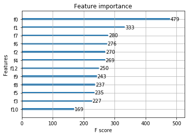
您可以使用 plotting(绘图)模块来绘制出 importance(重要性)以及输出的 tree(树).如果需要直接输出重要程度排名的话,则可以使用get_score方法或者get_fscore方法,两者不同之处在于前者可以通过importance_type参数添加权重。
要绘制出 importance(重要性), 可以使用 plot_importance. 该函数需要安装 matplotlib.
xgb.plot_importance(bst_with_evallist_and_early_stopping_100)
<matplotlib.axes._subplots.AxesSubplot at 0x7f2707a6a080>
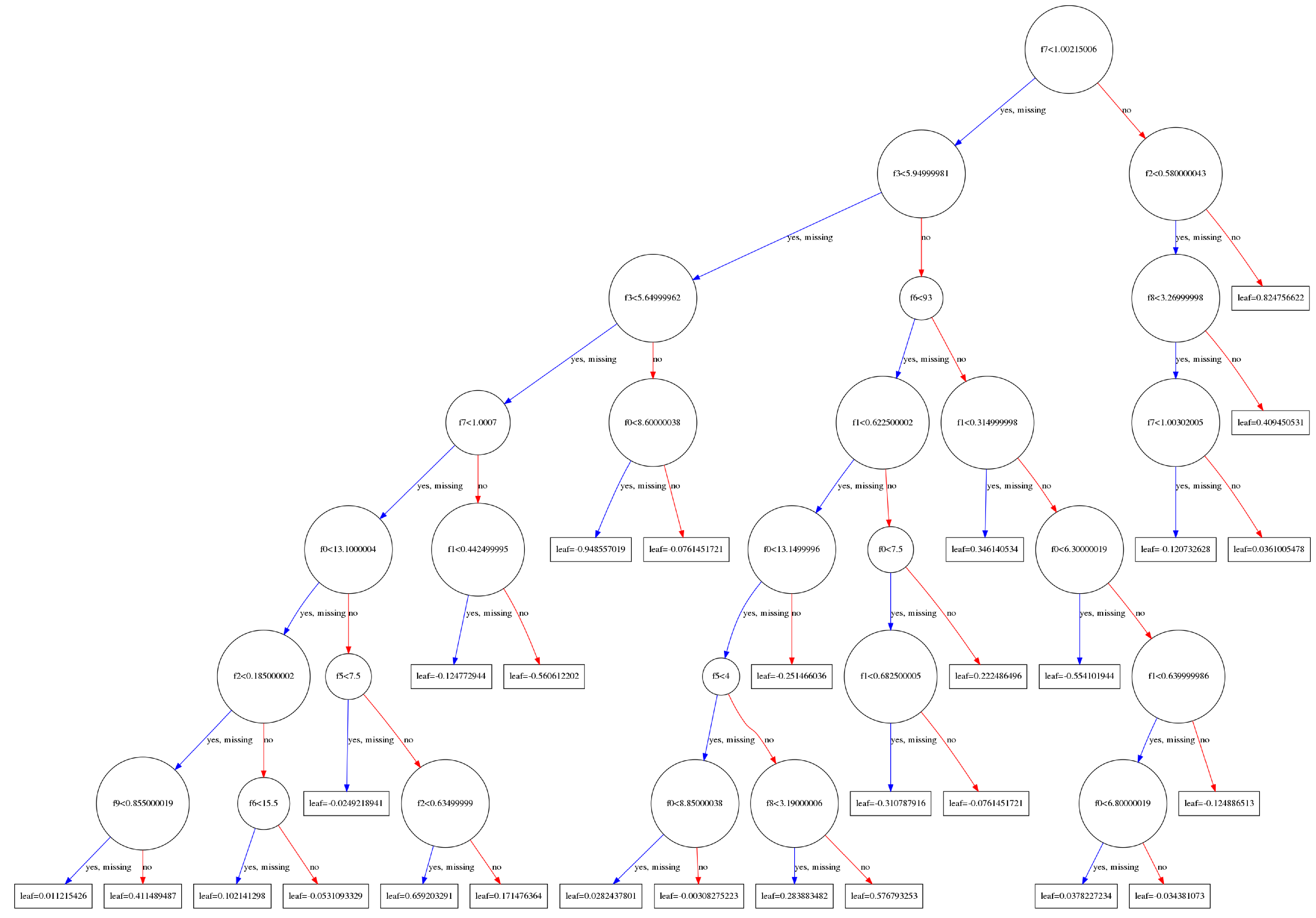
输出的 tree(树)会通过 matplotlib 来展示, 使用 plot_tree 指定 target tree(目标树)的序号. 该函数需要 graphviz 和 matplotlib.而且有一点要注意的是graphviz不仅仅是需要通过pip install graphviz来安装,还需要在你的系统中安装该软件,否则xgboost中的该部分将无法使用。此处可以参考我的另外一篇文章
除此之外我们还需要为plot_tree输入一个 matplotlib的ax,以控制输出图片的尺寸。
# xgb.plot_tree(bst, num_trees=2)
xgb.to_graphviz(bst_with_evallist_and_early_stopping_100, num_trees=2)
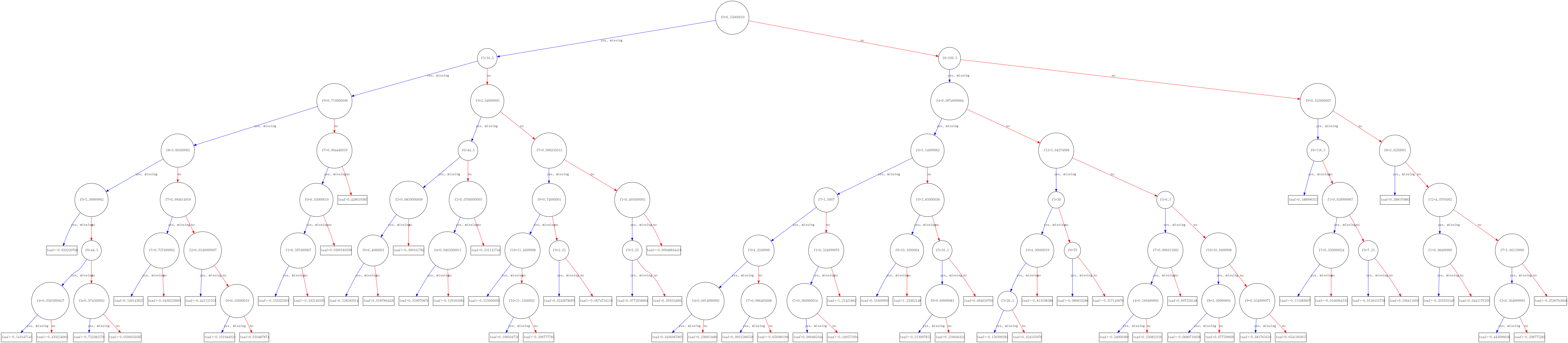
import matplotlib.pyplot as plt
fig = plt.figure()
ax = fig.add_axes([18.5,18.5,10.5,10.5])
xgb.plot_tree(bst_with_evallist_and_early_stopping_100, num_trees=2,ax=ax)
plt.show()