“不必遗憾。若是美好,叫做精彩。若是糟糕,叫做经历。”
2018年的最后一天
希望今年所有的遗憾,都是明年惊喜的铺垫!
致所有努力的人~
将KF、EKF、UKF在自动驾驶传感器融合当中的应用整理下吧:
卡尔曼滤波(KF)、扩展卡尔曼滤波(EKF)、无损卡尔曼滤波(UKF)
首先要搞清楚两个问题:1. 为什么要用KF、EKF、UKF?
2. 什么是KF、EKF、UKF?
先从最简单的KF说起吧~
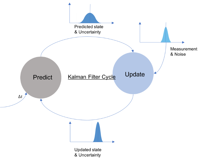
由于传感器本身的局限性以及自然界存在的噪声影响,导致我们依据传感器获取的任何测量结果都是有误差的,也就是我们通常无法精确的知道物体当前的状态。因此我们为了估计一个事物的状态,往往会去测量它,但是我们不能完全相信我们的测量,因为我们的测量是不精准的,它往往会存在一定的噪声,这个时候就需要在传感器测量结果的基础上,对目标的运动状态进行跟踪估计,以此来保证障碍物的位置、速度等信息不会发生突变而且是准确的。
KF、EKF以及UKF则是几种结合预测(先验分布)和测量更新(似然)的状态估计算法。这些算法能够应用于目标状态估计(目标可以是行人,车辆、GPS数据等)。
具体介绍KF的例程,网上的资料太多了,在此就不细说了,其实总的来说就3部分:初始化,预测,测量更新。
推荐两个网址:1. 知乎的陈光大神:https://zhuanlan.zhihu.com/p/45238681
2. AdamShan博客专家:https://blog.csdn.net/AdamShan/article/details/78248421
核心公式:
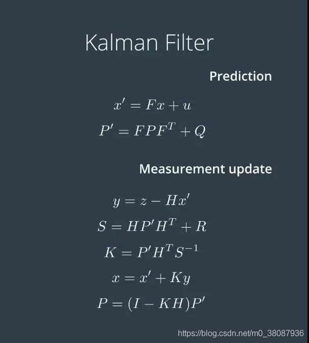
对于KF来讲,比较简单,而且Opencv里也有对应的cv::KalmanFilter模块,可以直接使用,其实它内部实现也是根据以上核心共式来封装的;当然也可以自己实现,下面就分别两种方法给出代码:
1.使用opencv里封装好的写的一个.hpp
/**************************************************************************
 * @author z.h
 * @date 2018.12.28
 * usage:kalman_filter_cv.hpp //opencv
 *
 **************************************************************************/

#ifndef KALMAN_FILTER_CV_H
#define KALMAN_FILTER_CV_H

#include <opencv2/opencv.hpp>

class kalman_filter_cv
{
public:
	kalman_filter_cv();
	~kalman_filter_cv();

	void _init(std::vector<float> v, int _mode)
	{
		if(_mode == 4)
		{
			state_num = 4;
			measure_num = 2;

			kf.init(state_num, measure_num, 0);
			kf.transitionMatrix = (cv::Mat_<float>(state_num, state_num) <<
				1, 0, 1, 0,
				0, 1, 0, 1,
				0, 0, 1, 0,
				0, 0, 0, 1);

			setIdentity(kf.measurementMatrix, cv::Scalar::all(1));
			setIdentity(kf.processNoiseCov, cv::Scalar::all(1e-5));
			setIdentity(kf.measurementNoiseCov, cv::Scalar::all(1));
			setIdentity(kf.errorCovPost, cv::Scalar::all(1));

			kf.statePost.at<float>(0, 0) = v[0];
			kf.statePost.at<float>(1, 0) = v[1];
			kf.statePost.at<float>(2, 0) = 0;
			kf.statePost.at<float>(3, 0) = 0;
		}
		else if(_mode == 8)
		{
			state_num = 8;
			measure_num = 4;

			kf.init(state_num, measure_num, 0);

			kf.transitionMatrix = (cv::Mat_<float>(state_num, state_num) <<
				1, 0, 0, 0, 1, 0, 0, 0,
				0, 1, 0, 0, 0, 1, 0, 0,
				0, 0, 1, 0, 0, 0, 1, 0,
				0, 0, 0, 1, 0, 0, 0, 1,
				0, 0, 0, 0, 1, 0, 0, 0,
				0, 0, 0, 0, 0, 1, 0, 0,
				0, 0, 0, 0, 0, 0, 1, 0,
				0, 0, 0, 0, 0, 0, 0, 1);

			setIdentity(kf.measurementMatrix, cv::Scalar::all(1));
			setIdentity(kf.processNoiseCov, cv::Scalar::all(1e-3));
			setIdentity(kf.measurementNoiseCov, cv::Scalar::all(1e-2));
			setIdentity(kf.errorCovPost, cv::Scalar::all(1));

			kf.statePost.at<float>(0, 0) = v[0];
			kf.statePost.at<float>(1, 0) = v[1];
			kf.statePost.at<float>(2, 0) = v[2];
			kf.statePost.at<float>(3, 0) = v[3];
			kf.statePost.at<float>(4, 0) = 0;
			kf.statePost.at<float>(5, 0) = 0;
			kf.statePost.at<float>(6, 0) = 0;
			kf.statePost.at<float>(7, 0) = 0;

		}
	}

	std::vector<float> _predict()
	{
		std::vector<float> res;
		cv::Mat state_ = kf.predict();

		for(int i = 0; i < state_.rows; ++i)
		{
			res.push_back(state_.at<float>(i,0));
		}
		return res;
	}

	void _correct(std::vector<float> v, int _mode)
	{
		if(_mode == 4)
		{
			cv::Mat measure_m = (cv::Mat_<float>(measure_m, 1) << v[0], v[1]);
			kf.correct(measure_m);
		}
		else if(_mode == 8)
		{
			cv::Mat measure_m = (cv::Mat_<float>(measure_m, 1) << v[0], v[1], v[2], v[3]);
			kf.correct(measure_m);
		}
	}

private:
	cv::KalmanFilter kf;
	int mode;
	int state_num;
	int measure_num;


};

#endif
2. 自己手写实现KF( kf.h and kf.cpp )
/**************************************************************************
 * @author z.h
 * @date 2018.xx.xx
 * @usage:kf.h
 * @brief:@params[IN]:@return:
 **************************************************************************/
#ifndef KF_H_KF_H
#define KF_H_KF_H

#include <opencv2/opencv.hpp>
#include <Eigen/Dense>

class kf
{
public:

	/**
	* Constructor
	*/
	kf();

	/**
	* Destructor
	*/
	virtual ~kf();

	/**
	* Init Initializes Kalman filter
	* @param x_in Initial state
	* @param P_in Initial state covariance
	* @param F_in Transition matrix
	* @param Q_in Process covariance matrix
	* @param H_in Measurement matrix
	* @param R_in Measurement covariance matrix
	*/
	void Init(Eigen::VectorXd &x_in, Eigen::MatrixXd &P_in, Eigen::MatrixXd &F_in,
			  Eigen::MatrixXd &Q_in, Eigen::MatrixXd &H_in, Eigen::MatrixXd &R_in);

	/**
	* Prediction Predicts the state and the state covariance
	*/
	void Predict();


	/**
	* Update Updates the state by using Standard Kalman Filter equations
	* @param z The measurement at k+1
	*/
	void Update(const Eigen::VectorXd &z);

	/**
	* Update Updates the state by using Extended Kalman Filter equations
	* @param z The measurement at k+1
	*/
	virtual void Update_ekf(const Eigen::VectorXd &z) = 0;


protected:

	// state vector
	Eigen::VectorXd x_;

	// state covariance matrix
	Eigen::MatrixXd P_;

	// state transistion matrix
	Eigen::MatrixXd F_;

	// process covariance matrix
	Eigen::MatrixXd Q_;

	// measurement matrix
	Eigen::MatrixXd H_;

	// measurement covariance matrix
	Eigen::MatrixXd R_;


};

#endif /* KF_H_KF_H */
/**************************************************************************
* @author z.h
* @date 2018.xx.xx
* @usage:kf.cpp
* @brief:@params[IN]:@return:
**************************************************************************/
#include <iostream>
#include "kf.h"
using Eigen::MatrixXd;
using Eigen::VectorXd;
const double PI = 3.141592653589793238463;
const float EPS = 0.0001;
kf::kf() {}
kf::~kf() {}
void kf::Init(VectorXd &x_in, MatrixXd &P_in, MatrixXd &F_in,
MatrixXd &Q_in, MatrixXd &H_in, MatrixXd &R_in){
x_ = x_in;
P_ = P_in;
F_ = F_in;
Q_ = Q_in;
H_ = H_in;
R_ = R_in;
}
void kf::Predict(){
/**
TODO:
* predict the state
*/
x_ = F_ * x_;
P_ = F_ * P_ * F_.transpose() + Q_;
}
void kf::Update(const VectorXd &z) {
/**
TODO:
* update the state by using Kalman Filter equations
*/
VectorXd y = z - H_ * x_;
/**
* @param y adjusted between -pi and pi;
*/
while (y(1) < -PI) {y(1) += 2 * PI;}
while (y(1) > PI) {y(1) += 2 * PI;}
MatrixXd S = H_ * P_ * H_.transpose() + R_;
MatrixXd K = P_ * H_.transpose() * S.inverse();
x_ = x_ + (K * y);
long size = x_.size();
MatrixXd I = MatrixXd::Identity(size,size);
P_ = (I - K * H_) * P_;
}
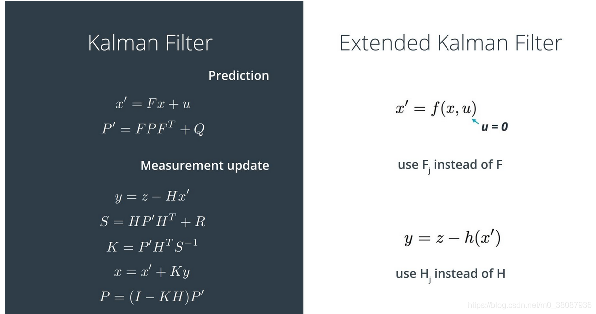
KF 这么好,但是一个最大的问题是只支持线性的,也就是它假设测量值在真值附近成高斯分布的,即高斯分布的x预测后仍服从高斯分布,高斯分布的x变换到测量空间后仍服从高斯分布。可是,假如F、H是非线性变换,那么上述条件则不成立,而且实际应用中哪有什么线性的情况,于是就引入了EKF,说白了,EKF就是KF的扩展,将实际中的非线性系统通过泰勒展开的形式线性化,以此利用KF。
数学中,泰勒公式是一个用函数在某点的信息描述其附近取值的公式。如果函数足够平滑的话,在已知函数在某一点的各阶导数值的情况之下,泰勒公式可以用这些导数值做系数构建一个多项式来近似函数在这一点的邻域中的值。
当然,EKF最经典的应用莫过于Lidar 与Radar的数据融合了
推荐一个github模板: https://github.com/asterixds/ExtendedKalmanFilter
但是,实际应用还需要修改,且不说运动状态模型的选择,数据的形式也是不同的,就拿Radar的数据来说吧,大陆的ARS-408-21其实提供的是笛卡尔坐标系下的数据,包括apollo 的融合也是用笛卡尔坐标系下的数据来做的,所以根本不需要用到EKF,当然还需根据实际情况来用。
下面给出(ekf.h and ekf.cpp)
/**************************************************************************
 * @author z.h
 * @date 2018.xx.xx
 * @usage:ekf.h
 * @brief:@params[IN]:@return:
 **************************************************************************/
#ifndef EKF_H_EKF_H
#define EKF_H_EKF_H

#include <iostream>
#include "kf.h"
#include "Eigen/Dense"
#include <vector>
#include <string>
#include <fstream>


class ekf:public kf
{
public:

	/**
    * Constructor.
    */
	ekf();

	/**
	* Destructor
	*/
	~ekf();

	/**
	* Update Updates the state by using Extended Kalman Filter equations
	* @param z The measurement at k+1
	*/
	void Update_ekf(const Eigen::VectorXd &z);

	/**
	* A helper method to calculate RMSE.
	*/
	Eigen::VectorXd CalculateRMSE(const vector<VectorXd> &estimations, const vector<VectorXd> &ground_truth);

	/**
	* A helper method to calculate Jacobians.
	*/
	Eigen::MatrixXd CalculateJacobian(const VectorXd& x_state);

	/**
	* ProcessFusion the main part of ekf
	*/
	void ProcessFusion(const SensorType &sensor_type_);

private:

	// check whether the tracking toolbox was initiallized or not (first measurement)
	bool is_initialized_;

	//acceleration noise
	float noise_ax, noise_ay;

	// previous timestamp
	long long previous_timestamp_;
    // present timestamp
	long long present_timestamp_;

	Eigen::MatrixXd R_lidar_;
	Eigen::MatrixXd R_radar_;
	Eigen::MatrixXd H_lidar_;
	Eigen::MatrixXd Hj_;

	enum SensorType{
	    LIDAR,
	    RADAR
    };

	Eigen::VectorXd raw_measurements_;


};


#endif /*EKF_H_EKF_H*/
/**************************************************************************
* @author z.h
* @date 2018.xx.xx
* @usage:ekf.cpp
* @brief:@params[IN]:@return:
**************************************************************************/
#include <iostream>
#include "ekf.h"
using Eigen::MatrixXd;
using Eigen::VectorXd;
/**
* Constructor.
*/
ekf::ekf()
{
// initializing matrices
is_initialized_ = false;
previous_timestamp_ = 0;
// Set the noise components
noise_ax = 9.f;
noise_ay = 9.f;
//measurement covariance matrix - lidar
R_lidar_ = MatrixXd(2, 2);
R_lidar_ << 0.0225, 0,
0, 0.0225;
//measurement covariance matrix - radar
R_radar_ = MatrixXd(3, 3);
R_radar_ << 0.09, 0, 0,
0, 0.0009, 0,
0, 0, 0.09;
//H matrix - lidar
H_lidar_ = MatrixXd(2, 4);
H_lidar_ << 1, 0, 0, 0,
0, 1, 0, 0;
//Hj_ jacobi matrix - radar
Hj_ = MatrixXd(3, 4);
Hj_ << 1, 1, 0, 0,
1, 1, 0, 0,
1, 1, 1, 1;
// Set the initial transition matrix F_
F_ = MatrixXd(4,4);
F_ << 1, 0, 1, 0,
0, 1, 0, 1,
0, 0, 1, 0,
0, 0, 0, 1;
//process uncertainty matrix
P_ = MatrixXd(4, 4);
P_ << 1, 0, 0, 0,
0, 1, 0, 0,
0, 0, 1000, 0,
0, 0, 0, 1000;
//state vector
x_ = VectorXd(4);
x_ << 1, 1, 1, 1;
}
/**
* Destructor.
*/
ekf::~ekf() {}
void ekf::Update_ekf(const Eigen::VectorXd &z)
{
/**
TODO:
* update the state by using Extended Kalman Filter equations
*/
double px = x_[0];
double py = x_[1];
double vx = x_[2];
double vy = x_[3];
double rho = sqrt(px*px + py*py );//range
double phi = 0;//bearing
double rho_dot = 0;//v
if (fabs(rho) > EPS) {
phi = atan2(py , px);// return value between -pi and pi
rho_dot = ((px * vx + py * vy) / rho);
}
VectorXd z_pred(3);
z_pred << rho, phi, rho_dot;
VectorXd y = z - z_pred;
while (y(1) < -PI) {y(1) += 2 * PI;}
while (y(1) > PI) {y(1) -= 2 * PI;}
MatrixXd S = H_ * P_ * H_.transpose() + R_;
MatrixXd K = P_ * H_.transpose() * S.inverse();
x_ = x_ + (K * y);
long size = x_.size();
MatrixXd I = MatrixXd::Identity(size,size);
P_ = (I - K * H_) * P_;
}
VectorXd ekf::CalculateRMSE(const vector<VectorXd> &estimations,
const vector<VectorXd> &ground_truth)
{
/**
TODO:
* Calculate the RMSE here.
*/
VectorXd rmse(4);
rmse << 0,0,0,0;
// estimation vector len should be non-zero and equal ground truth vector len
if(estimations.size() != ground_truth.size()
|| estimations.size() == 0){
cout << "Invalid estimation or ground_truth data" << endl;
return rmse;
}
//calculate squared errors
for(unsigned int i=0; i < estimations.size(); ++i){
VectorXd errors = estimations[i] - ground_truth[i];
errors = errors.array()*errors.array(); //coefficient-wise multiplication
rmse += errors;
}
//calculate the mean square root
rmse = rmse/estimations.size();
rmse = rmse.array().sqrt();
//return the result
return rmse;
}
MatrixXd CalculateJacobian(const VectorXd& x_state)
{
/**
TODO:
* Calculate a Jacobian here.
*/
MatrixXd Hj = MatrixXd::Zero(3, 4);
//recover state parameters
float px = x_state(0);
float py = x_state(1);
float vx = x_state(2);
float vy = x_state(3);
float c1 = px*px+py*py;
//check division by zero
if(fabs(c1) < EPS){
cout << "c1 = " << c1 << endl;
cout << "CalculateJacobian () - Error - Division by Zero" << endl;
return Hj;
}
float c2 = sqrt(c1);
float c3 = (c1*c2);
//compute the Jacobian
Hj << (px/c2), (py/c2), 0, 0,
-(py/c1), (px/c1), 0, 0,
py*(vx*py - vy*px)/c3, px*(px*vy - py*vx)/c3, px/c2, py/c2;
return Hj;
}
void ekf::ProcessFusion(const SensorType &sensor_type_ )
{
/****************************************************************************
* Initialization *
****************************************************************************/
if (!is_initialized_) {
/**
* Initialize the state ekf_.x_ with the first measurement.
* Create the covariance matrix.
* Remember: you'll need to convert radar from polar to cartesian coordinates.
*/
if (sensor_type_ == RADAR) {
/**
Convert radar from polar to cartesian coordinates and initialize state.
*/
double rho = raw_measurements_[0];
double phi = raw_measurements_[1];
double rho_dot = raw_measurements_[2];
x_ << rho*cos(phi), rho*sin(phi), 0, 0;
}
else if (sensor_type_ == LIDAR) {
/**
Initialize state.
*/
x_ << raw_measurements_[0], raw_measurements_[1], 0, 0;
}
previous_timestamp_ = present_timestamp_;
is_initialized_ = true;
return;
}
/****************************************************************************
* Prediction *
****************************************************************************/
/**
TODO:
* Update the state transition matrix F according to the new elapsed time.
- Time is measured in seconds.
* Update the process noise covariance matrix.
* Use noise_ax = 9 and noise_ay = 9 for your Q matrix.
*/
double dt = (present_timestamp_ - previous_timestamp_) / 1000000.0;
previous_timestamp_ = measurement_pack.timestamp_;
//Include delta time into the F matrix
F_(0, 2) = dt;
F_(1, 3) = dt;
if (dt>0){
float dt_2 = dt * dt;
float dt_3 = dt_2 * dt;
float dt_4 = dt_3 * dt;
//set the process covariance matrix Q
Q_ = MatrixXd(4, 4);
Q_ << dt_4/4*noise_ax, 0, dt_3/2*noise_ax, 0,
0, dt_4/4*noise_ay, 0, dt_3/2*noise_ay,
dt_3/2*noise_ax, 0, dt_2*noise_ax, 0,
0, dt_3/2*noise_ay, 0, dt_2*noise_ay;
Predict();
}
/****************************************************************************
* Update *
****************************************************************************/
/**
TODO:
* Use the sensor type to perform the update step.
* Update the state and covariance matrices.
*/
if (sensor_type_ == RADAR) {
// Radar updates
R_ = R_radar_;
H_ = CalculateJacobian(x_);
UpdateEKF(raw_measurements_);
} else {
// Laser updates
R_ = R_lidar_;
H_ = H_lidar_;
Update(raw_measurements_);
}
// print the output
cout << "x_ = " << x_ << endl;
cout << "P_ = " << P_ << endl;
}好嘞,我们已经知道KF不适用于非线性系统,为了处理非线性系统,通过一阶泰勒展式来近似(用线性函数近似),这个方案直接的结果就是,我们对于具体的问题都要求解对应的一阶偏导(雅可比矩阵),求解雅可比矩阵本身就是费时的计算,所以一种相对简单的状态估计算法——UKF就出现了。
UKF使用的是统计线性化技术,我们把这种线性化的方法叫做无损变换(unscented transformation)这一技术主要通过n个在先验分布中采集的点(我们把它们叫sigma points)的线性回归来线性化随机变量的非线性函数,由于我们考虑的是随机变量的扩展,所以这种线性化要比泰勒级数线性化(EKF所使用的策略)更准确。和EKF一样,UKF也主要分为预测和更新。
具体例程和代码参考:https://blog.csdn.net/AdamShan/article/details/78359048
끝났다.
加油啊!
2019,会转运吗