#一、准备
为了更深入的理解神经网络,笔者基本采用纯C++的手写方式实现,其中矩阵方面的运算则调用opencv,数据集则来自公开数据集a1a。
实验环境:
本文紧跟上篇文章深度学习实践(一)——logistic regression。
#二、神经网络基础
标准的神经网络结构如下图所示,其实就是上文logistic regression的增强版(即多加了几个隐层),基本思路还未变化。关于更详细的原理介绍,这里还是推荐吴恩达的深度学习系列课程。
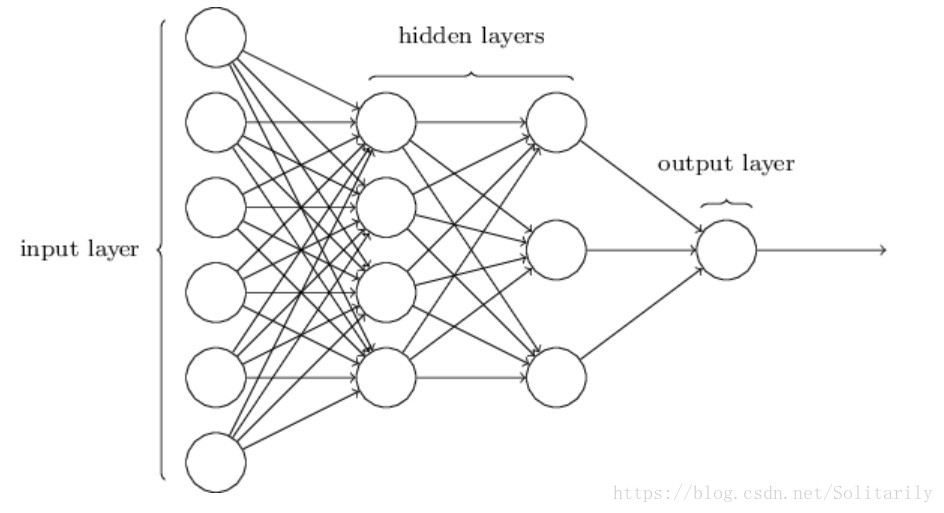
下面以三层神经网络(即上图)并结合a1a数据集,介绍构建的一般步骤:
- 初始化参数w1、w2、w3和b1、b2、b3,因为a1a数据集的维度是有123个特征,所以上图中input_layer维度为(123,m),m为样本数量,如训练集则为1065;而我们所构建的三层神经网络中间隐层神经元个数分别为(64,16,1),所以初始化参数矩阵w1(123,64)、w2(64,16)、w3(16,1)和偏置实数b1、b2、b3。
- 将W和X相乘(矩阵相乘,X为上层的输出,一开始即为样本的输入),再加上偏置b(为实数),则得到Z。
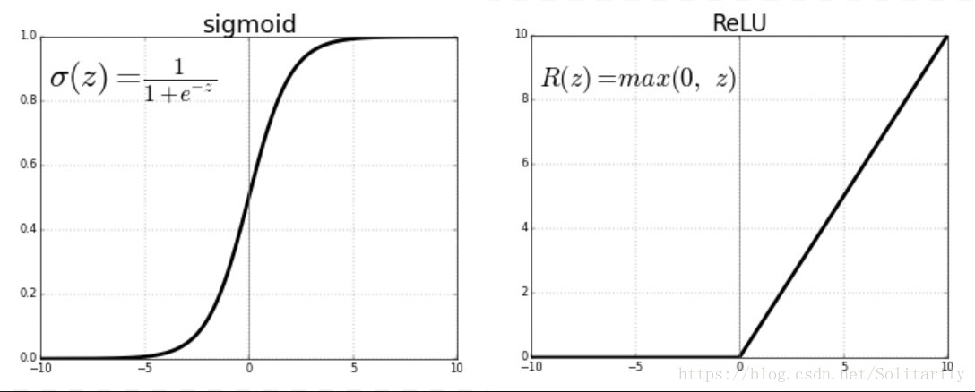
- 将Z进行激活,在隐层选择激活函数relu(可以更好的防止梯度爆炸,且结果很好),输出层选择sigmoid限制输出,它们的图像如下:
- 将上面的正向传播完成后,定义损失函数,这里使用交叉熵代价函数。
- 反向传播,并更新参数。
正向传播基本公式:
这里上标L代表第几层,上标i表示第几个样本(对应到a1a数据集即第几行),如
A[0]表示0层的输入(即样本输入)。
Z[1]=W[1]A[0]+b[1](1)
A[1]=Relu(Z[1])(2)
Z[2]=W[2]A[1]+b[2](3)
A[2]=Relu(Z[2])(4)
Z[3]=W[3]A[2]+b[3](5)
A[3]=Sigmoid(Z[3])(6)
L(A[3],Y^)=−A[3]log(A[3])−(1−Y^)log(1−A[3])(7)
The cost is then computed by summing over all training examples:
J=m1i=1∑mL(A(i)[3],Y(i))(8)
反向传播基本公式:
dA[3]=∂A[3]∂L=1−A[3]1−Y^−A[3]Y^(1)
dZ[3]=∂A[3]∂L∗∂Z[3]∂A[3]=dA[3]∗A[3]∗(1−A[3])(2)
dW[3]=∂Z[3]∂L∗∂W[3]∂Z[3]=m1dZ[3]A[2]T(3)
db[3]=∂Z[3]∂L∗∂b[3]∂Z[3]=m1i=1∑mdZ[3](i)(4)
dA[2]=∂Z[3]∂L∗∂A[2]∂Z[3]=W[3]TdZ[3](5)
dZ[2]=∂A[2]∂L∗∂Z[2]∂A[2]=dA[2]∗(A[2]>0)(6)
dW[2]=∂Z[2]∂L∗∂W[2]∂Z[2]=m1dZ[2]A[1]T(7)
db[2]=∂Z[2]∂L∗∂b[2]∂Z[2]=m1i=1∑mdZ[2](i)(8)
dA[1]=∂Z[2]∂L∗∂A[1]∂Z[2]=W[2]TdZ[2](9)
dZ[1]=∂A[1]∂L∗∂Z[1]∂A[1]=dA[1]∗(A[1]>0)(10)
dW[1]=∂Z[1]∂L∗∂W[1]∂Z[1]=m1dZ[1]A[0]T(11)
db[1]=∂Z[1]∂L∗∂b[1]∂Z[1]=m1i=1∑mdZ[1](i)(12)
#三、实践
数据集介绍、处理及一些公用的函数已在系列的上一篇文章,故在此不做赘述(只写出函数声明)。
从文件中创建矩阵:
void creatMat(Mat &x, Mat &y, String fileName);
初始化参数(这里使用xavier初始化):
void initial_parermaters(Mat &w, double &b, int n1, int n0) {
	w = Mat::zeros(n1, n0, CV_64FC1);
	b = 0.0;

	//double temp = 2 / (sqrt(n1));
	double temp = sqrt(6.0 / (double)(n1 + n0));
	RNG rng;
	for (int i = 0; i < w.rows; i++) {
		for (int j = 0; j < w.cols; j++) {
			w.at<double>(i, j) = rng.uniform(-temp, temp);//xavier初始化
														  //w.at<double>(i, j) = 0;
		}
	}
}
relu函数的编写:
void relu(const Mat &original, Mat &response) {
	response = original.clone();//防止维度不同
	for (int i = 0; i < original.rows; i++) {
		for (int j = 0; j < original.cols; j++) {
			if (original.at<double>(i, j) < 0) {
				response.at<double>(i, j) = 0.0;
			}
		}
	}
}
正向传播:
void linear_activation_forward(Mat &a_prev, Mat &a, Mat &w, double &b, string activation) {
	cv::Mat z;
	if (activation == "sigmoid") {
		z = (w*a_prev) + b;
		//cout << w.rows<<","<<w.cols<<" " << a_prev.rows<<","<<a_prev.cols<<endl;

		sigmoid(z, a);
	}
	else if (activation == "relu") {
		z = (w*a_prev) + b;
		//cout << w.rows << "," << w.cols << " " << a_prev.rows << "," << a_prev.cols << endl;

		relu(z, a);
	}
}
反向传播:
void activation_backward(const Mat &a, const Mat &da, Mat &dz, string activation) {
	if (activation == "sigmoid") {

		dz = da.mul(a.mul(1 - a));
	}
	else if (activation == "relu") {
		dz = da.clone();//保证维度相同
		for (int i = 0; i < a.rows; i++) {
			for (int j = 0; j < a.cols; j++) {
				if (a.at<double>(i, j) <= 0) {
					dz.at<double>(i, j) = 0.0;
				}
			}
		}
	}

}

void linear_backward(const Mat &da, const Mat &a, const Mat &a_prev, Mat &w, double &b, Mat &dw, double &db, Mat &da_prev, const int m, const double learning_rate, string activation) {
	cv::Mat dz;
	activation_backward(a, da, dz, activation);//激活函数的反向传播

	dw = (1.0 / m)*dz*a_prev.t();
	db = (1.0 / m)*sum(dz)[0];
	da_prev = w.t()*dz;
	w = w - (learning_rate * dw);
	b = b - (learning_rate * db);
}
#四、实验结果分析
迭代8000次cost分析:

我们容易发现更高的学习率可以获得较低的cost值,但是当其迭代到一定次数时,会有一定的起伏。
迭代8000次,准确率分析:

通过上图,易发现在一定迭代次数后,训练集和测试集准确率都会产生起伏,而且当训练集准确率不断上升时,测试集却未增长反而下降,最终产生了过拟合现象。
#五、结语
神经网络层数深,参数多,所以很难训练,一般训练8000次所需时间很长,下面的一篇文章主要讲一些优化方法(如adam),及如何处理过拟合(如dropout)等。
实验地址:码云