github:https://github.com/google-research/bert
解读翻译:https://www.jiqizhixin.com/articles/2018-11-01-9
https://baijiahao.baidu.com/s?id=1616001262563114372&wfr=spider&for=pc
https://zhuanlan.zhihu.com/p/34781297《attention is all you need》解读
https://blog.csdn.net/weixin_39470744
总结前篇的核心:
任务一:Masked LM
- 80% 的时间:用 [Mask] token 掩盖之前选择的单词。例如:
my dog is hairy→my dog is [Mask]. - 10% 的时间:用随机单词掩盖这个单词。例如:
my dog is hairy→my dog is apple. - 10% 的时间:保持单词不被掩盖。例如:
my dog is hairy→my dog is hairy.(这样做的目的是将表征偏向于实际观察到的单词)
任务二:Next Sentence Prediciton
- Input =
[CLS] the man went to [MASK] store [SEP] he bought a gallon [MASK] milk [SEP] - Label =
IsNext - Input =
[CLS] the man [MASK] to the store [SEP] penguin [MASK] are flight ##less birds [SEP] - Label =
NotNext
transformer模型部分 : Kyubyong实现版的解读
# -*- coding: utf-8 -*-
#/usr/bin/python2
'''
June 2017 by kyubyong park.
[email protected].
https://www.github.com/kyubyong/transformer
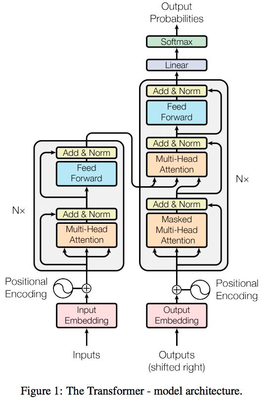
transfermer主要结构是由encoder和decoder构成。其中,encoder是由embedding + positional_encoding作为输入,
然后加一个dropout层,然后输入放到6个multihead_attention构成的结构中,每个multihead_attention后面跟一个feedforward。
而decoder是由decoder embedding + positional_encoding作为输入,输入到dropout层,
然后后面跟六个self multihead_attention+ multihead_attention,最后后面跟一个feedward。最后加一个liner projection
https://blog.csdn.net/weixin_38569817/article/details/81357650?utm_source=blogxgwz3
https://www.jianshu.com/p/ef41302edeef
rivastava R K, Greff K, Schmidhuber J. Highway networks[J]. arXiv preprintarXiv:1505.00387, 2015
'''
from __future__ import print_function
import tensorflow as tf
import numpy as np
def normalize(inputs,
epsilon = 1e-8,
scope="ln",
reuse=None):
'''Applies layer normalization.
Args:
inputs: A tensor with 2 or more dimensions, where the first dimension has
`batch_size`.
epsilon: A floating number. A very small number for preventing ZeroDivision Error.
scope: Optional scope for `variable_scope`.
reuse: Boolean, whether to reuse the weights of a previous layer
by the same name.
Returns:
A tensor with the same shape and data dtype as `inputs`.
'''
with tf.variable_scope(scope, reuse=reuse):
inputs_shape = inputs.get_shape()
params_shape = inputs_shape[-1:]
mean, variance = tf.nn.moments(inputs, [-1], keep_dims=True)
beta= tf.Variable(tf.zeros(params_shape))
gamma = tf.Variable(tf.ones(params_shape))
normalized = (inputs - mean) / ( (variance + epsilon) ** (.5) )
outputs = gamma * normalized + beta
return outputs
def embedding(inputs,
vocab_size,
num_units,
zero_pad=True,
scale=True,
scope="embedding",
reuse=None):
'''Embeds a given tensor.
Args:
inputs: A `Tensor` with type `int32` or `int64` containing the ids
to be looked up in `lookup table`.
vocab_size: An int. Vocabulary size.
num_units: An int. Number of embedding hidden units.
zero_pad: A boolean. If True, all the values of the fist row (id 0)
should be constant zeros.
scale: A boolean. If True. the outputs is multiplied by sqrt num_units.
scope: Optional scope for `variable_scope`.
reuse: Boolean, whether to reuse the weights of a previous layer
by the same name.
Returns:
A `Tensor` with one more rank than inputs's. The last dimensionality
should be `num_units`.
For example,
```
import tensorflow as tf
inputs = tf.to_int32(tf.reshape(tf.range(2*3), (2, 3)))
outputs = embedding(inputs, 6, 2, zero_pad=True)
with tf.Session() as sess:
sess.run(tf.global_variables_initializer())
print sess.run(outputs)
>>
[[[ 0. 0. ]
[ 0.09754146 0.67385566]
[ 0.37864095 -0.35689294]]
[[-1.01329422 -1.09939694]
[ 0.7521342 0.38203377]
[-0.04973143 -0.06210355]]]
```
```
import tensorflow as tf
inputs = tf.to_int32(tf.reshape(tf.range(2*3), (2, 3)))
outputs = embedding(inputs, 6, 2, zero_pad=False)
with tf.Session() as sess:
sess.run(tf.global_variables_initializer())
print sess.run(outputs)
>>
[[[-0.19172323 -0.39159766]
[-0.43212751 -0.66207761]
[ 1.03452027 -0.26704335]]
[[-0.11634696 -0.35983452]
[ 0.50208133 0.53509563]
[ 1.22204471 -0.96587461]]]
```
'''
with tf.variable_scope(scope, reuse=reuse):
lookup_table = tf.get_variable('lookup_table', #name
dtype=tf.float32,
shape=[vocab_size, num_units], #形状
initializer=tf.contrib.layers.xavier_initializer())
#print(lookup_table) #<tf.Variable 'encoder/enc_embed/lookup_table:0' shape=(9796, 512) dtype=float32_ref>
#<tf.Variable 'decoder/dec_embed/lookup_table:0' shape=(8767, 512) dtype=float32_ref>
if zero_pad:
lookup_table = tf.concat((tf.zeros(shape=[1, num_units]),
lookup_table[1:, :]), 0)
#print(lookup_table) #Tensor("decoder/dec_embed/concat:0", shape=(8767, 512), dtype=float32)
#Tensor("encoder/enc_embed/concat:0", shape=(9796, 512), dtype=float32)
outputs = tf.nn.embedding_lookup(lookup_table, inputs)
if scale:
outputs = outputs * (num_units ** 0.5)
#print(outputs) #shape=(32, 10, 512)
return outputs
def positional_encoding(inputs,
num_units,
zero_pad=True,
scale=True,
scope="positional_encoding",
reuse=None):
'''Sinusoidal Positional_Encoding.
Args:
inputs: A 2d Tensor with shape of (N, T).
num_units: Output dimensionality
zero_pad: Boolean. If True, all the values of the first row (id = 0) should be constant zero
scale: Boolean. If True, the output will be multiplied by sqrt num_units(check details from paper)
scope: Optional scope for `variable_scope`.
reuse: Boolean, whether to reuse the weights of a previous layer
by the same name.
Returns:
A 'Tensor' with one more rank than inputs's, with the dimensionality should be 'num_units'
'''
N, T = inputs.get_shape().as_list()
with tf.variable_scope(scope, reuse=reuse):
position_ind = tf.tile(tf.expand_dims(tf.range(T), 0), [N, 1])
# First part of the PE function: sin and cos argument
position_enc = np.array([
[pos / np.power(10000, 2.*i/num_units) for i in range(num_units)]
for pos in range(T)])
#print(position_enc)
# Second part, apply the cosine to even columns and sin to odds.
position_enc[:, 0::2] = np.sin(position_enc[:, 0::2]) # dim 2i
position_enc[:, 1::2] = np.cos(position_enc[:, 1::2]) # dim 2i+1
# Convert to a tensor
lookup_table = tf.convert_to_tensor(position_enc)
if zero_pad:
lookup_table = tf.concat((tf.zeros(shape=[1, num_units]),
lookup_table[1:, :]), 0)
outputs = tf.nn.embedding_lookup(lookup_table, position_ind)
if scale:
outputs = outputs * num_units**0.5
return outputs
def multihead_attention(queries,
keys,
num_units=None,
num_heads=8,
dropout_rate=0,
is_training=True,
causality=False,
scope="multihead_attention",
reuse=None):
'''Applies multihead attention.
Args:
queries: A 3d tensor with shape of [N, T_q, C_q].
keys: A 3d tensor with shape of [N, T_k, C_k].
num_units: A scalar. Attention size.
dropout_rate: A floating point number.
is_training: Boolean. Controller of mechanism for dropout.
causality: Boolean. If true, units that reference the future are masked.
num_heads: An int. Number of heads.
scope: Optional scope for `variable_scope`.
reuse: Boolean, whether to reuse the weights of a previous layer
by the same name.
Returns
A 3d tensor with shape of (N, T_q, C)
'''
with tf.variable_scope(scope, reuse=reuse):
# Set the fall back option for num_units
if num_units is None:
num_units = queries.get_shape().as_list[-1]
# print(num_units) #512
# Linear projections #全连接层
#print(queries) #shape=(32, 10, 512)
Q = tf.layers.dense(queries, num_units, activation=tf.nn.relu) # (N, T_q, C) #self.enc,
K = tf.layers.dense(keys, num_units, activation=tf.nn.relu) # (N, T_k, C) #self.enc,
V = tf.layers.dense(keys, num_units, activation=tf.nn.relu) # (N, T_k, C) #self.enc,
#print(Q) #shape=(32, 10, 512)
# Split and concat
Q_ = tf.concat(tf.split(Q, num_heads, axis=2), axis=0) # (h*N, T_q, C/h)
#print(Q_) #shape=(256, 10, 64) 拆成8个
K_ = tf.concat(tf.split(K, num_heads, axis=2), axis=0) # (h*N, T_k, C/h)
V_ = tf.concat(tf.split(V, num_heads, axis=2), axis=0) # (h*N, T_k, C/h)
# Multiplication
outputs = tf.matmul(Q_, tf.transpose(K_, [0, 2, 1])) # (h*N, T_q, T_k)
#print(outputs) #shape=(256, 10, 10)
# Scale
#print(K_.get_shape().as_list()[-1] ) #64
#print(K_.get_shape().as_list()) #[256, 10, 64]
outputs = outputs / (K_.get_shape().as_list()[-1] ** 0.5) #weight值
'''
key_masks它是想让那些key值的unit为0的key对应的attention score极小,这样在加权计算value的时候相当于对结果不造成影响。
首先用一个reduce_sum(keys, axis=-1))将最后一个维度上的值加起来,keys的shape也从[N, T_k, C_k]变为[N,T_k]
然后再用abs取绝对值,即其值只能为0,或正数
然后用到了tf.sign(x, name=None),该函数返回符号 y = sign(x) = -1 if x < 0; 0 if x == 0; 1 if x > 0,sign会将原tensor对应的每
个值变为-1,0,或者1。则经此操作,得到key_masks,有两个值,0或者1。0代表原先的keys第三维度所有值都为0,反之则为1,我们要mask的就是这些为0的key。
tf.tile把key_masks转化为shape为(h*N, T_k)的key_masks
每个queries都要对应这些keys,而mask的key对每个queries都是mask的。而之前的key_masks只相当于一份mask,所以扩充之前key_masks的维度,
在中间加上一个维度大小为queries的序列长度。然后利用tile函数复制相同的mask值即可。
定义一个和outputs同shape的paddings,该tensor每个值都设定的极小。
用where函数比较,当对应位置的key_masks值为0也就是需要mask时,outputs的该值(attention score)设置为极小的值(利用paddings实现),
否则保留原来的outputs值。
'''
# Key Masking
key_masks = tf.sign(tf.abs(tf.reduce_sum(keys, axis=-1))) # (N, T_k)
#print(keys) #(32, 10, 512)
#print(key_masks ) #shape=(32, 10)
key_masks = tf.tile(key_masks, [num_heads, 1]) # (h*N, T_k)
#print(key_masks) #shape=(256, 10) #8
key_masks = tf.tile(tf.expand_dims(key_masks, 1), [1, tf.shape(queries)[1], 1]) # (h*N, T_q, T_k)
#print(key_masks) #shape=(256, 10, 10) 在axes=1上增加一个维度
paddings = tf.ones_like(outputs)*(-2**32+1) #全1的矩阵,形状类似与outputs的形状
#print(paddings) ##shape=(256, 10, 10)
#tf.equal功能:对比两个矩阵/向量的元素是否相等,如果相等就返回True,反之返回False。
#where(condition, x=None, y=None, name=None)
#condition, x, y 相同维度,condition是bool型值,True/False where(condition)的用法,
#返回值,是condition中元素为True对应的索引
outputs = tf.where(tf.equal(key_masks, 0), paddings, outputs) # (h*N, T_q, T_k)
#等于0的位置是TRUE,其他的位置为False ,TRUE取padding中的值,false为outputs中的值
#print(outputs) #shape=(256, 10, 10) #8 * 64 ,10,10
# Causality = Future blinding
'''
causality参数告知我们是否屏蔽未来序列的信息(解码器self attention的时候不能看到自己之后的那些信息),这里即causality为True时的屏蔽操作。
'''
if causality:
diag_vals = tf.ones_like(outputs[0, :, :]) # (T_q, T_k)
#print(diag_vals) #shape=(10, 10)
#https://devdocs.io/tensorflow~python/tf/linalg/linearoperatorlowertriangular--线性代数库
'''
将该矩阵转为三角阵tril。三角阵中,对于每一个T_q,凡是那些大于它角标的T_k值全都为0,这样作为mask就可以让query只取它之前的key
(self attention中query即key)。由于该规律适用于所有query,接下来仍用tile扩展堆叠其第一个维度,构成masks,
shape为(h*N, T_q,T_k).------就是下三角矩阵,以上操作就可以当不需要来自未来的key值时将未来位置的key的score设置为极小
'''
tril = tf.linalg.LinearOperatorLowerTriangular(diag_vals).to_dense() # (T_q, T_k)
#print(tril) #shape=(10, 10)
masks = tf.tile(tf.expand_dims(tril, 0), [tf.shape(outputs)[0], 1, 1]) # (h*N, T_q, T_k)
#print(masks) #shape=(256, 10, 10)
#当不需要来自未来的key值时将未来位置的key的score设置为极小
paddings = tf.ones_like(masks)*(-2**32+1)
outputs = tf.where(tf.equal(masks, 0), paddings, outputs) # (h*N, T_q, T_k)
#print("-----")
# Activation 将attention score了利用softmax转化为加起来为1的权值,
outputs = tf.nn.softmax(outputs) # (h*N, T_q, T_k)
# Query Masking
'''
所谓要被mask的内容,就是本身不携带信息或者暂时禁止利用其信息的内容。这里query mask也是要将那些初始值为0的queryies
(比如一开始句子被PAD填充的那些位置作为query)mask住。代码前三行和key mask的方式大同小异,只是扩展维度等是在最后一个维度展开的。
操作之后形成的query_masks的shape为[h*N, T_q, T_k]。
第四行代码直接用outputs的值和query_masks相乘。这里的outputs是之前已经softmax之后的权值。所以此步之后,需要mask的权值会乘以0,
不需要mask的乘以之前取的正数的sign为1所以权值不变。实现了query_masks的目的。
这里源代码中的注释应该写错了,outputs的shape不应该是(N, T_q, C)而应该和query_masks 的shape一样,为(h*N, T_q, T_k)。
'''
query_masks = tf.sign(tf.abs(tf.reduce_sum(queries, axis=-1))) # (N, T_q)
query_masks = tf.tile(query_masks, [num_heads, 1]) # (h*N, T_q)
'''
由于每个queries都要对应这些keys,而mask的key对每个queries都是mask的。而之前的key_masks只相当于一份mask,所以扩充之前key_masks的维度,
在中间加上一个维度大小为queries的序列长度。然后利用tile函数复制相同的mask值即可。
'''
query_masks = tf.tile(tf.expand_dims(query_masks, -1), [1, 1, tf.shape(keys)[1]]) # (h*N, T_q, T_k)
#print(query_masks ) #shape=(256, 10, 10)
outputs *= query_masks # broadcasting. (N, T_q, C) #对应位置的元素相乘
'''
query mask也是要将那些初始值为0的queryies(比如一开始句子被PAD填充的那些位置作为query) mask住。
outputs的值和query_masks相乘。这里的outputs是之前已经softmax之后的权值。所以此步之后,需要mask的权值会乘以0,
不需要mask的乘以之前取的正数的sign为1所以权值不变。实现了query_masks的目的。
'''
#print(outputs) #shape=(256, 10, 10)
# Dropouts
outputs = tf.layers.dropout(outputs, rate=dropout_rate, training=tf.convert_to_tensor(is_training))
# Weighted sum
outputs = tf.matmul(outputs, V_) # ( h*N, T_q, C/h)
#print(V_) #shape=(256, 10, 64)
#print(outputs) #shape=(256, 10, 64)
# Restore shape
outputs = tf.concat(tf.split(outputs, num_heads, axis=0), axis=2 ) # (N, T_q, C)
#print(outputs) #shape=(32, 10, 512)
# Residual connection
outputs += queries #残差网络的思想
# Normalize
outputs = normalize(outputs) # (N, T_q, C)
#print(outputs) #shape=(32, 10, 512)
return outputs
def feedforward(inputs,
num_units=[2048, 512],
scope="multihead_attention",
reuse=None):
'''Point-wise feed forward net.
Args:
inputs: A 3d tensor with shape of [N, T, C].
num_units: A list of two integers.
scope: Optional scope for `variable_scope`.
reuse: Boolean, whether to reuse the weights of a previous layer
by the same name.
Returns:
A 3d tensor with the same shape and dtype as inputs
'''
with tf.variable_scope(scope, reuse=reuse):
# Inner layer
params = {"inputs": inputs, "filters": num_units[0], "kernel_size": 1,
"activation": tf.nn.relu, "use_bias": True}
outputs = tf.layers.conv1d(**params)
# Readout layer
params = {"inputs": outputs, "filters": num_units[1], "kernel_size": 1,
"activation": None, "use_bias": True}
outputs = tf.layers.conv1d(**params)
# Residual connection
outputs += inputs
# Normalize
outputs = normalize(outputs)
return outputs
#把之前的one_hot中的0改成了一个很小的数,1改成了一个比较接近于1的数
def label_smoothing(inputs, epsilon=0.1):
'''Applies label smoothing. See https://arxiv.org/abs/1512.00567.
Args:
inputs: A 3d tensor with shape of [N, T, V], where V is the number of vocabulary.
epsilon: Smoothing rate.
For example,
```
import tensorflow as tf
inputs = tf.convert_to_tensor([[[0, 0, 1],
[0, 1, 0],
[1, 0, 0]],
[[1, 0, 0],
[1, 0, 0],
[0, 1, 0]]], tf.float32)
outputs = label_smoothing(inputs)
with tf.Session() as sess:
print(sess.run([outputs]))
>>
[array([[[ 0.03333334, 0.03333334, 0.93333334],
[ 0.03333334, 0.93333334, 0.03333334],
[ 0.93333334, 0.03333334, 0.03333334]],
[[ 0.93333334, 0.03333334, 0.03333334],
[ 0.93333334, 0.03333334, 0.03333334],
[ 0.03333334, 0.93333334, 0.03333334]]], dtype=float32)]
```
'''
K = inputs.get_shape().as_list()[-1] # number of channels
return ((1-epsilon) * inputs) + (epsilon / K)
模型配置的参数:
" attention_probs_dropout_prob": 0.1, #乘法attention时,softmax后dropout概率
"hidden_act": "gelu", #激活函数
 "hidden_dropout_prob": 0.1, #隐藏层dropout概率
 "hidden_size": 768, #隐藏单元数
 "initializer_range": 0.02, #初始化范围
"intermediate_size": 3072, #升维维度
"max_position_embeddings": 512, #一个大于seq_length的参数,用于生成position_embedding "num_attention_heads": 12, #每个隐藏层中的attention head数
 "num_hidden_layers": 12, #隐藏层数
 "type_vocab_size": 2, #segment_ids类别 [0,1]
"vocab_size": 30522 #词典中词数
这里的输入参数:input_ids,input_mask,token_type_ids对应上篇文章中输出的input_ids,input_mask,segment_ids
transformer:
由于 Self-Attention 是每个词和所有词都要计算 Attention,所以不管他们中间有多长距离,最大的路径长度也都只是 1。可以捕获长距离依赖关系
attention表示成k、q、v的方式:
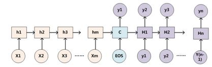
传统的attention(sequence2sequence问题):

上下文context表示成如下的方式(h的加权平均):

那么权重alpha(attention weight)可表示成Q和K的乘积,小h即V(下图中很清楚的看出,Q是大H,K和V是小h):

上述可以做个变种,就是K和V不想等,但需要一一对应,例如:
- V=h+x_embedding
- Q = H
- k=h
乘法VS加法attention
加法注意力:
还是以传统的RNN的seq2seq问题为例子,加性注意力是最经典的注意力机制,它使用了有一个隐藏层的前馈网络(全连接)来计算注意力分配:

乘法注意力:
就是常见的用乘法来计算attention score:
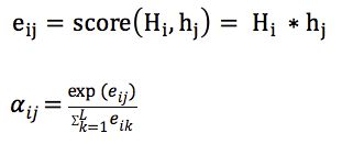
乘法注意力不用使用一个全连接层,所以空间复杂度占优;另外由于乘法可以使用优化的矩阵乘法运算,所以计算上也一般占优。
论文中的乘法注意力除了一个scale factor:
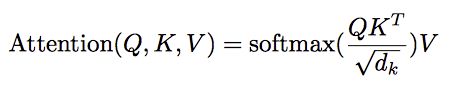
论文中指出当dk比较小的时候,乘法注意力和加法注意力效果差不多;但当d_k比较大的时候,如果不使用scale factor,则加法注意力要好一些,因为乘法结果会比较大,容易进入softmax函数的“饱和区”,梯度较小。

self-attention
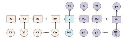
以一般的RNN的S2S为例子,一般的attention的Q来自Decoder(如下图中的大H),K和V来自Encoder(如下图中的小h)。self-attention就是attention的K、Q、V都来自encoder或者decoder,使得每个位置的表示都具有全局的语义信息,有利于建立长依赖关系。
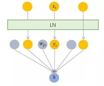
Layer normalization(LN)
batch normalization是对一个每一个节点,针对一个batch,做一次normalization,即纵向的normalization:

layer normalization(LN),是对一个样本,同一个层网络的所有神经元做normalization,不涉及到batch的概念,即横向normalization:
BN适用于不同mini batch数据分布差异不大的情况,而且BN需要开辟变量存每个节点的均值和方差,空间消耗略大;而且 BN适用于有mini_batch的场景。
LN只需要一个样本就可以做normalization,可以避免 BN 中受 mini-batch 数据分布影响的问题,也不需要开辟空间存每个节点的均值和方差。
但是,BN 的转换是针对单个神经元可训练的——不同神经元的输入经过再平移和再缩放后分布在不同的区间,而 LN 对于一整层的神经元训练得到同一个转换——所有的输入都在同一个区间范围内。如果不同输入特征不属于相似的类别(比如颜色和大小,scale不一样),那么 LN 的处理可能会降低模型的表达能力。
encoder:
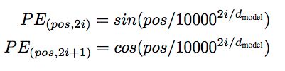
- 输入:和conv s2s类似,词向量加上了positional embedding,即给位置1,2,3,4...n等编码(也用一个embedding表示)。然后在编码的时候可以使用正弦和余弦函数,使得位置编码具有周期性,并且有很好的表示相对位置的关系的特性(对于任意的偏移量k,PE[pos+k]可以由PE[pos]表示):
- 输入的序列长度是n,embedding维度是d,所以输入是n*d的矩阵
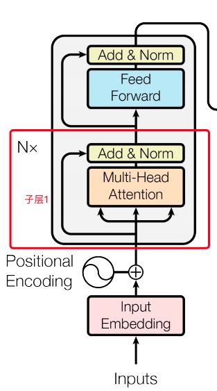
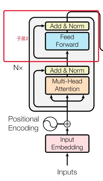
- N=6,6个重复一样的结构,由两个子层组成:
- 子层1:
- Multi-head self-attention
- 残余连接和LN:
- Output = LN (x+sublayer(x))
- 子层1:
-
- 子层2:
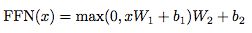
- Position-wise fc层(跟卷积很像)
- 对n*d的矩阵的每一行进行操作(相当于把矩阵每一行铺平,接一个FC),同一层的不同行FC层用一样的参数,不同层用不同的参数(对于全连接的节点数目,先从512变大为2048,再缩小为512):
- 子层2:

- 整个encoder的输出也是n*d的矩阵
decoder:
•输入:假设已经翻译出k个词,向量维度还是d
•同样使用N=6个重复的层,依然使用残余连接和LN
•3个子层,比encoder多一个attention层,是Decoder端去attend encoder端的信息的层:
- Sub-L1:
self-attention,同encoder,但要Mask掉未来的信息,得到k*d的矩阵

- Sub-L2:和encoder做attention的层,输出k*d的矩阵
- Sub-L3:全连接层,输出k*d的矩阵,用第k行去预测输出y
mutli-head attention:
MultiHead可以看成是一种ensemble方式,获取不同子空间的语义:


获取每个子任务的Q、K、V:
- 通过全连接进行线性变换映射成多个Q、K、V,线性映射得到的结果维度可以不变、也可以减少(类似降维)
- 或者通过Split对Q、K、V进行划分(分段)
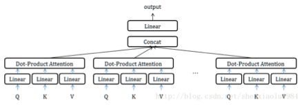
如果采用线性映射的方式,使得维度降低;或者通过split的方式使得维度降低,那么多个head做attention合并起来的复杂度和原来一个head做attention的复杂度不会差多少,而且多个head之间做attention可以并行。
decoder的输入:
self.y的输出
[[1008 3936 1924    4  401 5087 5651    3    0    0]
 [ 141   25    4  101 3180    6  362  552    3    0]
 [  15    4  420   12  845    3    0    0    0    0]
 [  79  243    6    1   15   42 1614  634    3    0]
 [ 527  119   30   85  976    3    0    0    0    0]
 [   1   12  669  193   20  135    1 7288    3    0]
 [   1    1    1    1    3    0    0    0    0    0]
 [  78   58    5 1934  764   87    3    0    0    0]
 [  65   20   44  484  304 1190    3    0    0    0]
 [  92  132    8 3174    5 1286  217    3    0    0]
 [ 534    1   81  979 2304    3    0    0    0    0]
 [  15  334   54   44  505  145    8  222 3052    3]
 [2124 2626 1435   14    3    0    0    0    0    0]
 [ 291  429   39    3    0    0    0    0    0    0]
 [   1    6  438  162    8  178 5506  702    3    0]
 [ 166  106   11   21    5  102 1403   97    3    0]
 [  47  578  116   18  387    3    0    0    0    0]
 [  11  100    5  173   28    1  459    3    0    0]
 [ 193   14   12    3    0    0    0    0    0    0]
 [  80  910   12 1581 1713    3    0    0    0    0]
 [  65   90  807    5   66   56    3    0    0    0]
 [  24   95   44 3973   85  340  327  110    3    0]
 [   1    1    1 1615    1    3    0    0    0    0]
 [  15   14   74  174   31    4 2982  512 1105    3]
 [ 350    3    0    0    0    0    0    0    0    0]
 [  96  246  425    5   54    3    0    0    0    0]
 [3585 1357  117 1105    1   61 5155    3    0    0]
 [  79  159    8    1  898    3    0    0    0    0]
 [  79   33   40  352    3    0    0    0    0    0]
 [  79 3060  569    6  515   25    1   39    3    0]
 [ 120   94  955   10   56 1606    3    0    0    0]
 [  24   95   28   16  139    7  244  199  729    3]]
self.dec:
[[[-2.279155    1.0991251  -1.5886356  ...  1.4294004  -1.5982031
   -1.1408417 ]
  [-1.5231744  -0.05949117 -1.1321675  ... -1.4490161  -0.30499786
   -0.77806205]
  [-1.3187622  -0.15014127 -1.13905    ... -3.1452506  -2.686214
   -0.5845207 ]
  ...
  [-0.41217917  1.4415227  -1.2828536  ... -0.3612737  -0.4510218
   -0.7630521 ]
  [-0.7186153   0.86343354 -1.883712   ... -0.91078717 -0.01014436
    0.07463718]
  [-0.86691934  0.98398304 -2.3404958  ... -0.8095867   0.442111
   -0.04082058]]

 [[-2.631531    0.8046703  -1.8410189  ...  0.98089796 -1.0553441
   -1.0271642 ]
  [-2.527477    0.47748724 -1.5274042  ... -0.9979782  -1.4225875
self.x德语 [[ 14 29 1 111 744 3 0 0 0 0]
[ 344 303 3 0 0 0 0 0 0 0]
[ 352 68 13 22 2974 1 1 3 0 0]
[ 37 68 459 591 8 9 94 3 0 0]
[ 100 210 70 737 3 0 0 0 0 0]
[ 34 1 4 3720 492 119 1 2668 3 0]
[ 21 6 660 1234 116 25 4757 539 1 3]
[ 832 12 46 160 154 32 3 0 0 0]
[ 34 7 20 1067 1 3 0 0 0 0]
[ 25 207 19 18 2361 1 28 3 0 0]
[ 34 1 2921 1123 3 0 0 0 0 0]
[ 34 1 5514 10 56 1 3 0 0 0]
[ 61 14 110 78 8 19 334 3 0 0]
[ 21 15 420 356 3 0 0 0 0 0]
[ 14 171 3183 310 2075 2426 1024 3 0 0]
[ 65 362 13 35 1 10 217 4820 3 0]
[ 25 75 8 557 124 2810 2124 9 29 3]
[ 774 1 1 1 3 0 0 0 0 0]
[ 1 7 1149 4973 3 0 0 0 0 0]
[ 21 11 99 19 2640 107 215 3 0 0]
[ 163 1116 29 1335 402 9 197 3 0 0]
[ 120 2161 918 157 15 23 6 400 1335 3]
[ 21 11 174 89 1260 9 86 71 3 0]
[ 14 48 4 3168 111 54 45 375 3 0]
[ 34 617 225 23 465 3 0 0 0 0]
[ 95 886 12 3115 1 3 0 0 0 0]
[ 340 269 12 16 426 874 1797 156 117 3]
[ 204 28 4 3979 30 8 2287 30 1 3]
[ 477 52 10 405 3787 168 902 51 3 0]
[ 100 28 4 1241 98 2820 1 3 0 0]
[ 14 589 27 64 1 3 0 0 0 0]
self.y英语 [[ 1 27 13 134 4 1534 3332 3 0 0]
[5502 7 349 8 701 8414 114 3 0 0]
[ 125 101 444 2134 2960 1767 10 480 2865 3]
[ 120 21 143 4641 1866 7 1149 3 0 0]
[ 291 12 33 2686 3 0 0 0 0 0]
[ 92 55 1 955 3 0 0 0 0 0]
[1540 9 1 7 1 3 0 0 0 0]
[3050 37 4 462 502 12 8718 3 0 0]
[ 11 100 13 5 29 559 3 0 0 0]
[ 125 175 48 73 12 169 4592 7722 3 0]
[5070 7 2667 47 1 3 0 0 0 0]
[ 231 12 41 1 57 1708 3 0 0 0]
[ 1 6 13 20 1 3 0 0 0 0]
[ 15 4 420 12 111 3 0 0 0 0]
[ 235 4 314 457 261 21 8 559 3722 3]
[ 15 115 2008 3 0 0 0 0 0 0]
[ 65 94 4087 17 160 3 0 0 0 0]
[ 11 3803 130 1 1661 1 4 4373 3 0]
[ 49 1 9 332 303 110 3 0 0 0]
[ 1 162 6 4 614 181 100 17 3 0]
[ 24 11 182 4885 3 0 0 0 0 0]
[ 96 488 1 1 79 421 3 0 0 0]
[ 965 8 1126 28 20 13 1 3 0 0]
[ 120 63 784 5 2063 3565 3 0 0 0]
[ 24 16 132 5 174 9 4755 392 3 0]
[ 166 44 246 366 3 0 0 0 0 0]
[ 24 28 25 129 22 1411 3 0 0 0]
[ 737 298 3720 162 3 0 0 0 0 0]
[ 11 100 5 75 477 4 1054 3 0 0]
[ 65 164 25 156 1 46 8431 3 0 0]
[ 80 18 198 2343 624 3 0 0 0 0]
[ 640 281 37 162 3 0 0 0 0 0]]
deecoder部分:
[[ 2 24 334 54 164 25 2337 114 3 0]
[ 2 1 10 423 48 20 115 91 25 17]
[ 2 47 114 37 18 234 10 417 4175 10]
[ 2 166 1 121 3475 409 5 8 1 97]
[ 2 80 12 8 1924 901 159 8 7055 901]
[ 2 96 86 1 79 8 1 2252 3 0]
[ 2 2171 87 11 18 1 23 38 136 4969]
[ 2 120 1 1326 3555 3 0 0 0 0]
[ 2 79 345 7208 19 4 6423 3 0 0]
[ 2 589 16 21 263 5134 53 6 381 267]
[ 2 601 44 265 17 37 22 19 643 3]
[ 2 80 83 104 1242 3 0 0 0 0]
[ 2 141 12 9 2443 77 339 122 5 1571]
[ 2 4358 216 137 61 1 10 3 0 0]
[ 2 3130 1 1 3 0 0 0 0 0]
[ 2 96 181 242 9 89 3 0 0 0]
[ 2 65 20 19 1 4223 127 3 0 0]
[ 2 15 138 51 1303 23 50 1386 3 0]
[ 2 15 13 27 173 56 22 926 460 3]
[ 2 65 21 5 1942 9 3 0 0 0]
[ 2 79 8 51 143 676 4787 3 0 0]
[ 2 15 42 227 19 1225 3 0 0 0]
[ 2 15 16 63 5 286 131 6 8 4174]
[ 2 166 1 23 4 1 3 0 0 0]
[ 2 15 17 4367 12 3481 3562 7 298 1]
[ 2 15 11 100 38 377 5 29 23 13]
[ 2 15 981 112 18 1 8 1169 3 0]
[ 2 15 16 2135 523 1 3 0 0 0]
[ 2 4264 17 12 33 68 208 3 0 0]
[ 2 80 12 4 4979 1 3 0 0 0]
[ 2 11 823 13 51 109 3 0 0 0]
[ 2 79 33 1431 390 3 0 0 0 0]]
[ 25 1 201 526 3 0 0 0 0 0]]self.decoder_inputs的构成tf.concat((tf.ones_like(self.y[:, :1])*2, self.y[:, :-1]), -1)tf.ones_like(self.y[:, :1])
[[1]
[1]
[1]
[1]
[1]
[1]
[1]
[1]
[1]
[1]
[1]
[1]
[1]
[1]
[1]
[1]
[1]
[1]
[1]
[1]
[1]
[1]
[1]
[1]
[1]
[1]
[1]
[1]
[1]
[1]
[1]
[1]]
tf.ones_like(self.y[:, :1])*2
[[2]
[2]
[2]
[2]
[2]
[2]
[2]
[2]
[2]
[2]
[2]
[2]
[2]
[2]
[2]
[2]
[2]
[2]
[2]
[2]
[2]
[2]
[2]
[2]
[2]
[2]
[2]
[2]
[2]
[2]
[2]
[2]]
self.y[:, :-1]
[[ 11 74 123 350 95 41 3029 3 0]
[3510 144 3781 3 0 0 0 0 0]
[ 1 92 738 173 8 1 3 0 0]
[ 96 94 547 29 8 4941 1096 3 0]
[ 49 64 220 3 0 0 0 0 0]
[ 203 13 3 0 0 0 0 0 0]
[2917 1523 59 4 204 35 330 3 0]
[ 24 97 44 17 12 41 1 2429 87]
[ 79 4 985 4074 1143 557 3187 3 0]
[ 92 55 4 7987 3611 12 8 1578 37]
[ 24 4 212 806 12 159 1 3 0]
[1410 336 68 2515 3 0 0 0 0]
[ 150 28 194 29 2887 17 1 3 0]
[ 15 4 101 37 500 12 1 3 0]
[ 96 18 1 2972 43 11 139 14 3]
[2629 6333 2802 3 0 0 0 0 0]
[ 610 4 1 11 90 445 9 3 0]
[7991 138 10 1481 3 0 0 0 0]
[ 24 5119 122 10 4 360 984 3 0]
[6026 689 3 0 0 0 0 0 0]
[1033 34 9 1202 3 0 0 0 0]
[ 203 13 231 18 14 57 4 89 3]
[ 43 17 12 33 69 11 182 3 0]
[ 11 18 275 93 311 3 0 0 0]
[2016 22 84 4 1428 899 3 0 0]
[ 24 16 132 5 64 1493 25 1744 289]
[ 98 1298 3170 703 390 3 0 0 0]
[ 24 11 353 232 214 19 8 1 3]
[ 15 28 11 238 72 1850 54 3 0]
[ 203 13 3 0 0 0 0 0 0]
[ 231 278 9 489 12 33 53 48 3]
[ 600 12 878 5 1582 4 572 3 0]] #由原来的32*10变成了32*9
tf.concat((tf.ones_like(self.y[:, :1])*2, self.y[:, :-1]), -1)
[[ 2 394 33 1133 30 32 3 0 0 0]
[ 2 1675 28 13 64 3 0 0 0 0]
[ 2 15 4777 944 5 102 5 4 1871 3]
[ 2 291 12 33 2686 3 0 0 0 0]
[ 2 11 105 5707 3 0 0 0 0 0]
[ 2 11 119 4231 20 6 4 1577 1135 3]
[ 2 965 4 326 18 4762 3 0 0 0]
[ 2 284 967 111 1484 968 1622 3 0 0]
[ 2 15 6 191 3498 3 0 0 0 0]
[ 2 24 16 21 4 1 1 3 0 0]
[ 2 1160 101 91 20 159 1 3232 3 0]
[ 2 15 42 51 584 3 0 0 0 0]
[ 2 394 33 4681 3 0 0 0 0 0]
[ 2 80 12 41 448 5956 10 1 6524 3]
[ 2 98 416 2000 17 23 4 204 3 0]
[ 2 80 12 301 7 8061 3 0 0 0]
[ 2 284 1579 6 4 1 3 0 0 0]
[ 2 125 4 1385 88 6913 2257 20 25 162]
[ 2 2219 1346 3 0 0 0 0 0 0]
[ 2 67 12 490 28 124 260 5 34 3]
[ 2 47 315 177 12 1 3 0 0 0]
[ 2 6239 12 4 290 6 1 3 0 0]
[ 2 78 3 0 0 0 0 0 0 0]
[ 2 92 103 133 504 14 3 0 0 0]
[ 2 15 28 25 4 668 6 7226 2454 3]
[ 2 24 473 288 543 430 706 48 81 3]
[ 2 689 11 424 21 8420 6647 87 3 0]
[ 2 203 13 3 0 0 0 0 0 0]
[ 2 15 26 71 8 137 6 742 3 0]
[ 2 79 72 803 3 0 0 0 0 0]
[ 2 589 12 41 240 6 4 4257 3 0]
[ 2 15 39 6379 3 0 0 0 0 0]]
encoder的输入是德语部分,k,q都是德语句子本身,v也是本句,开始self-attention,最后形成的是self.encoder。
decoder的输入是英语部分,输入的是英语句子,但是第一个数值都换成了2,其余的10个数值不变,k,q,都是本身。最后形成self.decoder。同样是self-attention,
在decoder和encoder链接的地方进行普通的attention,q=self.decoder,k=self.encoder,v=self.encoder。 softmax(q*k/d)*v
标签y的输入是英语部分。
最后计算概率的一层shape=(32, 10, 8767),8767代表单词表的大小,最后给出的是对应概率最大的位置,与label对比,也就是和y对比。input_decoder做了特殊的处理:在decoder的输入中,self-attention的部分要进行对未来信息的屏蔽,用来预防看到未来的信息,起最终的屏蔽后的结果是一个下三角矩阵(10,10)
1 0 0 0 0 0 0 0 0 0
1 6 0 0 0 0 0 0 0 0
1 6 10 0 0 0 0 0 0 0
1 6 10 13 0 0 0 0 0 0
1 6 10 13 15 0 0 0 0 0
...........................................................其意思是有encoder端的一句10个词汇构成的语义向量并且配合矩阵第一行的第一个元素,预测出第二行的第二元素。
其实在预测阶段是没有decoder的输入的部分的,只有根据encode端预测decoder的第一个字符,然后根据encoder的端加上预测出的第一个字符,预测第二个字符,直到预测出第10个字符
import tensorflow as tf
a = tf.constant([[[2, 2, 12,22], [3, 3, 31,23],[3, 4, 5,6], [3, 9, 3,8]]], dtype=tf.float32)
diag_vals = tf.ones_like(a[0, :, :])
tril = tf.linalg.LinearOperatorLowerTriangular(diag_vals).to_dense()

sess = tf.Session()
print(sess.run(tril))


[[1. 0. 0. 0.]
 [1. 1. 0. 0.]
 [1. 1. 1. 0.]
 [1. 1. 1. 1.]]
对于decoder的self.attention部分:数据的变换如上面的程序将(10,10)的矩阵转换成下三角矩阵。
masks = tf.tile(tf.expand_dims(tril, 0), [tf.shape(outputs)[0], 1, 1])通过这条语句将形成(256,10,10)的结构,embedding=512,一句话有10个单词,mutihead=8,一个批次有32句话。
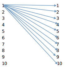
转换过程:(32,10,512)--8*(32,10,512/8)----8*(32,10,64)---(256,10,64)------->q*k---------(256,10,64)*(256,10,64)-----(256,10,10)---32句话,每句话有10个单词,按照将512的空间分解成64的空间,然后进行self.attention的计算得出该句话的每个单词同这句话的其他单词的权重如下图:1--10代表的是一句话中的10个单词,连线上是权重,是通过softmax函数计算出的。
key的处理部分:32句话,每句话10个人单词,(32,10,512)----最后一个维度相加得到(32,10),8个attention -----8个32*10,每个都是同样的。(256,10)----8个一组,最后是(256,10,10),同样的一句话变成了---------(8*32,10,10)以
a = tf.constant([[2, 2, 12,22],[3, 3, 31,23],[3, 4, 5,6]], dtype=tf.float32)  #3*4
tril = tf.tile(a,[8,1])
[[ 2.  2. 12. 22.]
 [ 3.  3. 31. 23.]
 [ 3.  4.  5.  6.]
 [ 2.  2. 12. 22.]
 [ 3.  3. 31. 23.]
 [ 3.  4.  5.  6.]
 [ 2.  2. 12. 22.]
 [ 3.  3. 31. 23.]
 [ 3.  4.  5.  6.]
 [ 2.  2. 12. 22.]
 [ 3.  3. 31. 23.]
 [ 3.  4.  5.  6.]
 [ 2.  2. 12. 22.]
 [ 3.  3. 31. 23.]
 [ 3.  4.  5.  6.]
 [ 2.  2. 12. 22.]
 [ 3.  3. 31. 23.]
 [ 3.  4.  5.  6.]
 [ 2.  2. 12. 22.]
 [ 3.  3. 31. 23.]
 [ 3.  4.  5.  6.]
 [ 2.  2. 12. 22.]
 [ 3.  3. 31. 23.]
 [ 3.  4.  5.  6.]]
tril = tf.tile(tf.expand_dims(tril, 1), [1, 2, 1]) #(24, 2, 4)
[[[ 2.  2. 12. 22.]
  [ 2.  2. 12. 22.]]

 [[ 3.  3. 31. 23.]
  [ 3.  3. 31. 23.]]

 [[ 3.  4.  5.  6.]
  [ 3.  4.  5.  6.]]

 [[ 2.  2. 12. 22.]
  [ 2.  2. 12. 22.]]

 [[ 3.  3. 31. 23.]
  [ 3.  3. 31. 23.]]

 [[ 3.  4.  5.  6.]
  [ 3.  4.  5.  6.]]

 [[ 2.  2. 12. 22.]
  [ 2.  2. 12. 22.]]

 [[ 3.  3. 31. 23.]
  [ 3.  3. 31. 23.]]

 [[ 3.  4.  5.  6.]
  [ 3.  4.  5.  6.]]

 [[ 2.  2. 12. 22.]
  [ 2.  2. 12. 22.]]

 [[ 3.  3. 31. 23.]
  [ 3.  3. 31. 23.]]

 [[ 3.  4.  5.  6.]
  [ 3.  4.  5.  6.]]

 [[ 2.  2. 12. 22.]
  [ 2.  2. 12. 22.]]

 [[ 3.  3. 31. 23.]
  [ 3.  3. 31. 23.]]

 [[ 3.  4.  5.  6.]
  [ 3.  4.  5.  6.]]

 [[ 2.  2. 12. 22.]
  [ 2.  2. 12. 22.]]

 [[ 3.  3. 31. 23.]
  [ 3.  3. 31. 23.]]

 [[ 3.  4.  5.  6.]
  [ 3.  4.  5.  6.]]

 [[ 2.  2. 12. 22.]
  [ 2.  2. 12. 22.]]

 [[ 3.  3. 31. 23.]
  [ 3.  3. 31. 23.]]

 [[ 3.  4.  5.  6.]
  [ 3.  4.  5.  6.]]
[[ 2.  2. 12. 22.]
  [ 2.  2. 12. 22.]]

 [[ 3.  3. 31. 23.]
  [ 3.  3. 31. 23.]]

 [[ 3.  4.  5.  6.]
  [ 3.  4.  5.  6.]]]
经过计算后变成了(8*32,10,10)其中第二个维度中的10代表了一个句子中的第一个单词重复10次,其他词也一样,然后进行权重与(10,10)的矩阵的相乘权重矩阵同样为10*10,代表的意思是第一行为,第一个单词同其他所有单词的权重,第二行为第二个单词和其他所有单词的权重,依次类推......................
[[25 55 95 36 34 88 47 19 35 84]
[23 82 51 11 79 34 73 90 37 23]
[47 4 4 21 3 77 72 9 29 26]
[47 96 34 49 27 71 4 86 73 24]
[92 99 85 37 44 67 28 67 90 30]
[73 23 34 47 88 48 33 54 79 77]
[87 79 45 56 58 25 16 60 77 22]
[19 8 67 96 84 31 13 21 76 61]
[49 5 56 7 75 0 12 9 56 93]
[72 99 56 3 2 79 52 70 17 79]]
padding
[[[-4.2949673e+09 -4.2949673e+09 -4.2949673e+09 -4.2949673e+09]
  [-4.2949673e+09 -4.2949673e+09 -4.2949673e+09 -4.2949673e+09]
  [-4.2949673e+09 -4.2949673e+09 -4.2949673e+09 -4.2949673e+09]
  [-4.2949673e+09 -4.2949673e+09 -4.2949673e+09 -4.2949673e+09]]
.....................................
masks = tf.tile(tf.expand_dims(tril, 0), [tf.shape(outputs)[0], 1, 1])主要是为了形成和shape(256,10,10)一样形状的张量,paddings = tf.ones_like(masks)*(-2**32+1),每个元素值都为-4.2949673e+09为最小值。outputs = tf.where(tf.equal(masks, 0), paddings, outputs)将(q×k)/(d^1/2),将其中为0的元素替换成-4.2949673e+09,outputs =tf.nn.softmax(outputs)
然后对query进行mask,
a = tf.constant([[2, 2, 12,-2],[3, 3, 31,0],[3, 4, 0,0]], dtype=tf.float32)  #3*4  batchsize = 3
query_masks = tf.sign(tf.abs(a))
[[1. 1. 1. 1.]
 [1. 1. 1. 0.]
 [1. 1. 0. 0.]]
key_masks维度的扩充是在 1上,query_masks的维度扩充是在-1上,也就是最后一个维度上。在msak的处理上,形成类似的张量,维度是在
[[[1. 0. 0. 0.]
  [1. 1. 0. 0.]
  [1. 1. 1. 0.]
  [1. 1. 1. 1.]]

 [[1. 0. 0. 0.]
  [1. 1. 0. 0.]
  [1. 1. 1. 0.]
  [1. 1. 1. 1.]]

 [[1. 0. 0. 0.]
  [1. 1. 0. 0.]
  [1. 1. 1. 0.]
  [1. 1. 1. 1.]]

 [[1. 0. 0. 0.]
  [1. 1. 0. 0.]
  [1. 1. 1. 0.]
  [1. 1. 1. 1.]]]
进行屏蔽后q×k/(d^1/2)的值类似于如下的输出
[[[ 2.0000000e-01 -4.2949673e+09 -4.2949673e+09 -4.2949673e+09]
  [ 5.1999998e-01  5.1999998e-01 -4.2949673e+09 -4.2949673e+09]
  [ 1.1200000e-01  1.1200000e-01  1.1200000e-01 -4.2949673e+09]
  [ 0.0000000e+00  0.0000000e+00  0.0000000e+00  0.0000000e+00]]

 [[ 4.3000001e-01 -4.2949673e+09 -4.2949673e+09 -4.2949673e+09]
  [ 3.0000001e-01  3.0000001e-01 -4.2949673e+09 -4.2949673e+09]
  [ 0.0000000e+00  0.0000000e+00  0.0000000e+00 -4.2949673e+09]
  [ 0.0000000e+00  0.0000000e+00  0.0000000e+00  0.0000000e+00]]

 [[ 3.0000001e-01 -4.2949673e+09 -4.2949673e+09 -4.2949673e+09]
  [ 4.0000001e-01  4.0000001e-01 -4.2949673e+09 -4.2949673e+09]
  [ 5.0000000e-01  5.0000000e-01  5.0000000e-01 -4.2949673e+09]
  [ 6.0000002e-01  6.0000002e-01  6.0000002e-01  6.0000002e-01]]

 [[ 8.9999998e-01 -4.2949673e+09 -4.2949673e+09 -4.2949673e+09]
  [ 4.3000001e-01  4.3000001e-01 -4.2949673e+09 -4.2949673e+09]
  [ 5.0999999e-01  5.0999999e-01  5.0999999e-01 -4.2949673e+09]
  [ 6.2000000e-01  6.2000000e-01  6.2000000e-01  6.2000000e-01]]]
成为了一个下三角矩阵,也就形成了对未来信息的屏蔽。
函数运行的例子
#-*-coding:utf-8-*-
import tensorflow as tf
# x = [[1,2,3],[4,5,6]]
# y = [[7,8,9],[10,11,12]]
# condition3 = [[True,False,False],
#              [False,True,True]]
# condition4 = [[True,False,False],
#              [True,False,False]]
# with tf.Session() as sess:
#     print(sess.run(tf.where(condition3,x,y)))
#     print(sess.run(tf.where(condition4,x,y)))

#shape=(2, 2, 3)
# a = tf.constant([[[2, 2, 12,22], [3, 3, 31,23]],[[3, 4, 5,6], [3, 9, 3,8]]], dtype=tf.int32)
# b = tf.constant([[1, 7], [2, 9]], dtype=tf.int32)
# c = tf.constant([[1, 11], [2, 12]], dtype=tf.float32)
# oneHot = tf.one_hot(a,depth=35)
# # print(a)
# # print(b)
# # print(c)
# # d = tf.matmul(b,c)
# # Q_ = tf.concat(tf.split(a, 2, axis=2),axis=0) # (h*N, T_q, C/h)
# # print(Q_)
# with tf.Session() as sess:
#     # print(sess.run(tf.split(a, 2, axis=2)))
#     # print(Q_ )
#     # print(sess.run(Q_))
#     print(sess.run(oneHot))#, [3, 3, 31,23],[3, 4, 5,6], [3, 9, 3,8]
a = tf.constant([[2, 2, 12,-2],[3, 3, 31,0],[3, 4, 0,0],[3, 9, 3,8]], dtype=tf.float32)  #3*4  batchsize = 3
q = tf.constant([[2, 2, 12,-2],[3, 3, 31,0],[3, 4, 0,0]], dtype=tf.float32)

diag_vals = tf.ones_like(a)
outputs =  tf.constant([[0.2, 0.52, 0.112,0],[0.43, 0.3, 0,0],[0.3, 0.4, 0.5,0.6],[0.9, 0.43, 0.51,0.62]], dtype=tf.float32)
tril = tf.linalg.LinearOperatorLowerTriangular(diag_vals).to_dense()
masks = tf.tile(tf.expand_dims(tril, 0), [tf.shape(tril)[0], 1, 1])
paddings = tf.ones_like(masks)*(-2**32+1)

#tril = tf.expand_dims(a, 0)
outputs = tf.tile(outputs,[1,1])
outputs =  tf.tile(tf.expand_dims(outputs, -1), [1, 1, 4])
# print(tf.Session().run(outputs))
# query_masks = tf.sign(tf.abs(q))
# query_masks = tf.tile(query_masks, [8, 1]) # (h*N, T_q)
# query_masks = tf.tile(tf.expand_dims(query_masks, -1), [1, 1, 4])

# tril = tf.tile(a,[8,1]) #(24,4)===(3*8,4)
# masks = tf.tile(tf.expand_dims(tril, 1), [1, 4, 1]) #(24, 2, 4)
#
# paddings = tf.ones_like(masks)*(-2**32+1)  #-4 294 967 295
#
# outputs = tf.where(tf.equal(masks, 0), paddings, outputs)
sess = tf.Session()
# # outputs = tf.where(tf.equal(masks, 0), paddings, outputs)
# outputs *=query_masks
print(sess.run(tf.where(tf.equal(masks, 0), paddings, outputs)))
# print(sess.run(tf.equal(masks, 0)))
# print("---",sess.run(outputs))

# import numpy as np
#
# num = []
# arr = np.random.random((10,10))
#
# print(arr)
最后的输出 outputs*v至此整个attention的过程结束。(在传统的attention中v和k表示的同一个句子,而q表示的是目标句子),在预测未来的目标语句时,对于目标语句中未来的信息,要进行屏蔽,避免影响。
self.target,留下非0 的是1 ,0的位置还是0
[[1. 1. 1. 1.]
 [1. 1. 1. 0.]
 [1. 1. 0. 0.]
 [1. 1. 1. 1.]]