大型在线零售商通常使用基于查询的搜索来帮助消费者在其网站上查找信息/产品。他们能够使用技术为用户提供更好的体验。因为他们了解搜索相关性的重要性,并且长时间和/或不成功的搜索可以将用户转移,因为用户已经习惯并期望即时,相关的搜索结果,例如他们从淘宝、京东获得的搜索结果。
虽然搜索对于任何电子商务业务的成功至关重要,但对于中小型在线零售商来说,搜索并不总是那么容易,因为它往往需要大量的手动标记数据和机器学习技术。
即使数据发生变化或结构不合理,查询也不准确,高质量搜索就是要返回相关结果。以下是我们今天要做的事情:仅将原始文本作为输入,我们的目标是预测Home Depot网站上产品与搜索结果的相关性,从而帮助他们改善客户的购物体验。
数据
数据集描述:
使用的如下三个表:
- train.csv 训练集,包括产品,搜索和相关性分数
- product_descriptions.csv 包括每个产品的文字说明
- attribute.csv 提供有关产品子集的扩展信息
这三个表中包含一下数据字段:
- id 唯一的Id字段,表示(search_term,product_uid)对
- product_uid 产品的ID
- product_title 产品名称
- product_description 产品的文本描述(可能包含HTML内容)
- search_term 搜索查询
- relevance 给定id的相关性评级的平均值(我们将针对给定的搜索词预测的特征)
- name 属性名称
- value 属性的值
数据处理
import numpy as np
import pandas as pd
from nltk.stem.porter import *
import re
import random
import warnings
warnings.filterwarnings('ignore')
random.seed(2018)
stemmer = PorterStemmer()
# 数据载入
train = pd.read_csv('train.csv', encoding="ISO-8859-1")
pro_desc = pd.read_csv('product_descriptions.csv')
attributes = pd.read_csv('attributes.csv')
# 从attributes中提取产品的品牌
brand = attributes.query('name == "MFG Brand Name"').iloc[:,[0,2]].rename(columns={'value':'brand'})
# 数据合成
df = train.merge(pro_desc, how='left', on='product_uid')
df = df.merge(brand, how='left', on='product_uid')
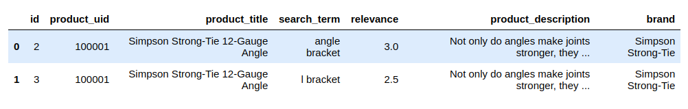
df.head(2)
文字预处理
文本处理是应用任何机器学习NLP算法之前的重要阶段。尽管文本处理在技术上可以在特征生成过程中完成,但我想先进行所有处理,然后再进行特征生成。这是因为相同的处理文本被用作输入以生成若干不同的特征。
- 搜索词拼写纠正(谷歌字典)
- 统一单位
- 删除特殊字符
- 词干文本
- 标记文
# 定义一个函数对字符类型数据处理
def str_stem(s):
    if isinstance(s, str):
        # 单位处理
        s = re.sub(r"([0-9])( *)\.( *)([0-9])", r"\1.\4", s)
        s = re.sub(r"([0-9]+)( *)(inches|inch|in|')\.?", r"\1in. ", s)
        s = re.sub(r"([0-9]+)( *)(foot|feet|ft|'')\.?", r"\1ft. ", s)
        s = re.sub(r"([0-9]+)( *)(pounds|pound|lbs|lb)\.?", r"\1lb. ", s)
        s = re.sub(r"([0-9]+)( *)(square|sq) ?\.?(feet|foot|ft)\.?", r"\1sq.ft. ", s)
        s = re.sub(r"([0-9]+)( *)(cubic|cu) ?\.?(feet|foot|ft)\.?", r"\1cu.ft. ", s)
        s = re.sub(r"([0-9]+)( *)(gallons|gallon|gal)\.?", r"\1gal. ", s)
        s = re.sub(r"([0-9]+)( *)(ounces|ounce|oz)\.?", r"\1oz. ", s)
        s = re.sub(r"([0-9]+)( *)(centimeters|cm)\.?", r"\1cm. ", s)
        s = re.sub(r"([0-9]+)( *)(milimeters|mm)\.?", r"\1mm. ", s)
        s = re.sub(r"([0-9]+)( *)(°|degrees|degree)\.?", r"\1 deg. ", s)
        s = re.sub(r"([0-9]+)( *)(v|volts|volt)\.?", r"\1 volt. ", s)
        s = re.sub(r"([0-9]+)( *)(wattage|watts|watt)\.?", r"\1 watt. ", s)
        s = re.sub(r"([0-9]+)( *)(amperes|ampere|amps|amp)\.?", r"\1 amp. ", s)
        s = re.sub(r"([0-9]+)( *)(qquart|quart)\.?", r"\1 qt. ", s)
        s = re.sub(r"([0-9]+)( *)(hours|hour|hrs.)\.?", r"\1 hr ", s)
        s = re.sub(r"([0-9]+)( *)(gallons per minute|gallon per minute|gal per minute|gallons/min.|gallons/min)\.?", r"\1 gal. per min. ", s)
        s = re.sub(r"([0-9]+)( *)(gallons per hour|gallon per hour|gal per hour|gallons/hour|gallons/hr)\.?", r"\1 gal. per hr ", s)
        # 处理特殊字符
        s = s.replace("$"," ")
        s = s.replace("?"," ")
        s = s.replace(" "," ")
        s = s.replace("&","&")
        s = s.replace("'","'")
        s = s.replace("/>/Agt/>","")
        s = s.replace("</a<gt/","")
        s = s.replace("gt/>","")
        s = s.replace("/>","")
        s = s.replace("<br","")
        s = s.replace("<.+?>","")
        s = s.replace("[ &<>)(_,;:!?\+^~@#\$]+"," ")
        s = s.replace("'s\\b","")
        s = s.replace("[']+","")
        s = s.replace("[\"]+","")
        s = s.replace("-"," ")
        s = s.replace("+"," ")
        # 删除括号中内容
        s = s.replace("[ ]?[[(].+?[])]","")
        # 删除 sizes
        s = s.replace("size: .+$","")
        s = s.replace("size [0-9]+[.]?[0-9]+\\b","")


        return " ".join([stemmer.stem(re.sub('[^A-Za-z0-9-./]', ' ', word)) for word in s.lower().split()])
    else:
        return "null"

# 处理文字数据,比较耗时
df['product_title'] = df['product_title'].apply(str_stem)
df['search_term'] = df['search_term'].apply(str_stem)
df['product_description'] = df['product_description'].apply(str_stem)
df['brand'] = df['brand'].apply(str_stem)
生成特征
任何机器学习项目中最重要也最耗时的部分就是特征工程,这里我们的主要特征是文本,新创建的特征可以分为几类:
- 计数特征:查询长度,标题长度,描述长度,品牌长度,查询和标题之间的相同的词,查询和描述之间的相同的词,以及查询和品牌之间的相同的词
举个例子,在搜索的时候我们搜索"shower only faucet",产品的相关标题”Delta Vero 1-Handle Shower Only Faucet Trim Kit in Chrome (Valve Not Included)“,相关产品说明是”Update your bathroom with the Delta Vero Single-Handle Shower Faucet Trim Kit in Chrome. It has a sleek, modern and minimalistic aesthetic. The MultiChoice universal valve keeps the water temperature within +/-3 degrees Fahrenheit to help prevent scalding.California residents: see Proposition 65 informationIncludes the trim kit only, the rough-in kit (R10000-UNBX) is sold separatelyIncludes the handleMaintains a balanced pressure of hot and cold water even when a valve is turned on or off elsewhere in the systemDue to WaterSense regulations in the state of New York, please confirm your shipping zip code is not restricted from use of items that do not meet WaterSense qualifications“
在此示例中,整个查询出现在产品标题中一次,整个查询未出现在产品说明中。
在同一个例子中,查询中出现的三个单词也出现在产品标题中,因此,查询和产品标题之间有三个相同的词。查询中出现的两个单词也出现在产品描述中,因此,查询和产品描述之间有两个相同的词,依此类推。
- 统计特征:标题长度与查询长度的比率,描述长度与查询长度的比率,标题和查询常用字数与查询长度的比率,描述和查询常用字数与查询长度的比率,查询与品牌常用字词的比率数到品牌长度
要创建新功能,我们需要创建几个函数来计算共同词和常用的整个术语数
# 创建统计关联词个数函数
def str_common_word(str1, str2):
    str1, str2 = str1.lower(), str2.lower()
    words, count = str1.split(), 0
    for word in words:
        if str2.find(word)>=0:
            count+=1
    return count

def str_whole_word(str1, str2, i_):
    str1, str2 = str1.lower().strip(), str2.lower().strip()
    count = 0
    while i_ < len(str2):
        i_ = str2.find(str1, i_)
        if i_ == -1:
            return count
        else:
            count += 1
            i_ += len(str1)
    return count

### 创建文本类特征
df['word_len_of_search_term'] = df['search_term'].apply(lambda x:len(x.split())).astype(np.int64)
df['word_len_of_title'] = df['product_title'].apply(lambda x:len(x.split())).astype(np.int64)
df['word_len_of_description'] = df['product_description'].apply(lambda x:len(x.split())).astype(np.int64)
df['word_len_of_brand'] = df['brand'].apply(lambda x:len(x.split())).astype(np.int64)
# 创建一个结合了“search_term”,“product_title”和“product_description”的新列
df['product_info'] = df['search_term']+"\t"+df['product_title'] +"\t"+df['product_description']
# 整个搜索词出现在产品标题中的次数
df['query_in_title'] = df['product_info'].map(lambda x:str_whole_word(x.split('\t')[0],x.split('\t')[1],0))
# 整个搜索词出现在产品说明中的次数
df['query_in_description'] = df['product_info'].map(lambda x:str_whole_word(x.split('\t')[0],x.split('\t')[2],0))
# 搜索词中出现的单词数也会出现在产品标题中
df['word_in_title'] = df['product_info'].map(lambda x:str_common_word(x.split('\t')[0],x.split('\t')[1]))
# 搜索词中出现的单词数也出现在制作说明中
df['word_in_description'] = df['product_info'].map(lambda x:str_common_word(x.split('\t')[0],x.split('\t')[2]))
# 产品标题字长与搜索字词长度的比率
df['query_title_len_prop']=df['word_len_of_title']/df['word_len_of_search_term']
# 产品描述字长与搜索字词长度的比率
df['query_desc_len_prop']=df['word_len_of_description']/df['word_len_of_search_term']
# 产品标题和搜索词常用字数与搜索字词数的比率
df['ratio_title'] = df['word_in_title']/df['word_len_of_search_term']
# 产品描述和搜索词常用词cout与搜索词词数的比率
df['ratio_description'] = df['word_in_description']/df['word_len_of_search_term']
# 创建新列结合了“search_term”,“brand”和“product_title”。
df['attr'] = df['search_term']+"\t"+df['brand']+"\t"+df['product_title']
# 搜索字词中出现的字数也会出现在品牌中。
df['word_in_brand'] = df['attr'].map(lambda x:str_common_word(x.split('\t')[0],x.split('\t')[1]))
# 搜索字词和品牌常用字数与品牌字数的比率
df['ratio_brand'] = df['word_in_brand']/df['word_len_of_brand']

# 删除不需要的列
df.drop(['id', 'product_uid', 'product_title', 'search_term', 'product_description', 'brand', 'product_info', 'attr'], axis=1, inplace=True)

### 可视化特征关联度
%matplotlib inline
import matplotlib.pyplot as plt
import seaborn as sns
corr = df.corr()
plt.figure(figsize=(10,8))
sns.heatmap(corr, cmap='cool')

建模
数据集创建
from sklearn.model_selection import train_test_split

from sklearn.model_selection import train_test_split
X = df.loc[:, df.columns != 'relevance']
y = df.loc[:, df.columns == 'relevance']
X_train, X_test, y_train, y_test = train_test_split(X, y, test_size=0.3, random_state=0)
随机森林回归模型
from sklearn.ensemble import RandomForestRegressor
from sklearn.metrics import mean_squared_error

rf = RandomForestRegressor(n_estimators=100, max_depth=6, random_state=0)
rf.fit(X_train, y_train.values.ravel())
y_pred = rf.predict(X_test)
rf_mse = mean_squared_error(y_pred, y_test)
rf_rmse = np.sqrt(rf_mse)
print('随机森林均方根偏差是(rmse):{:.4f}'.format(rf_rmse))
随机森林均方根偏差是(rmse):0.4790
岭回归模型
from sklearn.linear_model import Ridge

rg= Ridge(alpha=.1)
rg.fit(X_train, y_train.values.ravel())
y_pred = rg.predict(X_test)
rg_rmse = (mean_squared_error(y_pred, y_test)) ** 0.5
print('岭回归均方根偏差是(rmse):{:.4f}'.format(rg_rmse))
岭回归均方根偏差是(rmse):0.4852
梯度提升回归模型
from sklearn.ensemble import GradientBoostingRegressor

est = GradientBoostingRegressor(n_estimators=100, learning_rate=0.1, max_depth=1, random_state=0, loss='ls').fit(X_train, y_train.values.ravel())
y_pred = est.predict(X_test)
est_mse = mean_squared_error(y_pred, y_test)
est_rmse = np.sqrt(est_mse)
print('梯度提升回归模型均方根偏差是(rmse):{:.4f}'.format(est_rmse))
梯度提升回归模型均方根偏差是(rmse):0.4827
Xgboost回归模型
import xgboost

xgb = xgboost.XGBRegressor(n_estimators=100, learning_rate=0.08, gamma=0, subsample=0.75, colsample_bytree=1, max_depth=7)
xgb.fit(X_train, y_train.values.ravel())
y_pred = xgb.predict(X_test)
xgb_mse = mean_squared_error(y_pred, y_test)
xgb_rmse = np.sqrt(xgb_mse)
print('Xgboost回归模型均方根偏差是(rmse): %.4f' % xgb_rmse)
Xgboost回归模型均方根偏差是(rmse): 0.4776
结果
result = pd.DataFrame([[rf_rmse, rg_rmse, est_rmse, xgb_rmse]],
                      columns=['随机森林', '岭回归', '梯度提升回归', 'Xgboost']).T
result.columns = ['rmse']
result
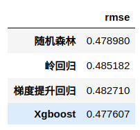
可见Xgboost效果最好,且性能比随机森林高
特征重要性
XGBoost库提供了一种称为内置函数plot_importance()来绘制由他们的重要性排序功能
from xgboost import plot_importance
plt.figure(figsize=(8,6))
plot_importance(xgb)

产品描述越详细,越方便被找到