目录
一、数据摸底
1.1 数据加载
数据下载路径:https://www.kaggle.com/c/titanic/data
import pandas as pd

data_train = pd.read_csv("../train.csv")
data_predict = pd.read_csv("../test.csv")

full = data_train.append(data_predict, ignore_index=True) #合并训练集和测试集,对特征统一处理
1.2 数据统计描述和可视化
1、数据类型查看
full.head()
类别变量:Cabin、Embarked、Pclass、Sex、Survived
连续数值变量:Age、Fare
离散数值变量:Parch、SibSp
2、特征缺失值查看
full.info()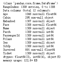
Cabin有77%的数据缺失,应舍弃;
Age有20%的数据缺失,考虑用平均值填充;
Fare、Embarked有几条数据缺失,分别考虑用平均值、众数填充。
3、变量统计描述
数值型变量统计描述
full.describe()
年龄在[65,80]的乘客占比1%,full['Age'].describe(percentiles=[0.98,0.99])
票价大于500的乘客占比小于1%,full['Fare'].describe(percentiles=[0.98,0.99])
没有携带父母和孩子的乘客占比75%;
在三等舱的乘客占比大约50%;
携带配偶的乘客占比大约30%;
类别变量统计描述
full.describe(include=['O'])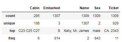
乘客登船地点有三个,主要集中在S站;
男性乘客占比64.4%。
4、特征变量与目标变量的相关性
类别变量与目标变量的相关性
data_train[['Pclass','Survived']].groupby(['Pclass'], as_index=False).mean().sort_values(by='Survived', ascending=False)
data_train[['Sex','Survived']].groupby(['Sex'], as_index=False).mean().sort_values(by='Survived', ascending=False)
data_train[['Embarked','Survived']].groupby(['Embarked'], as_index=False).mean().sort_values(by='Survived', ascending=False)
船舱级别越高,乘客的生还概率越大,P1>P2>P3;
女性乘客有更大的生存概率;
在C站上船的乘客有更大的生存概率。
离散数值变量与目标变量的相关性
data_train[['SibSp','Survived']].groupby(['SibSp'], as_index=False).mean().sort_values(by='Survived', ascending=False)
data_train[['Parch','Survived']].groupby(['Parch'], as_index=False).mean().sort_values(by='Survived', ascending=False)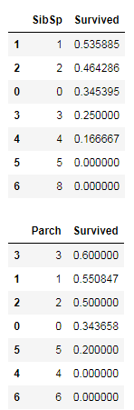
当家人(父母、子女、配偶、兄弟姐妹)数量达到一定值时,与目标变量的相关性为0,应构建一些组合的衍生变量。
连续数值变量与目标变量的相关性
import seaborn as sns
import matplotlib.pyplot as plt

g = sns.FacetGrid(data_train,col='Survived')
g.map(plt.hist, "Age", bins=16)
g = sns.FacetGrid(data_train,col='Survived')
g.map(plt.hist, "Fare", bins=10)
年龄:孩童(<=5)和老人(80)拥有更大的生还概率,15-25岁的乘客生还概率较小,乘客大多集中在15-35岁。
票价:票价<=50的乘客生还概率较小,当乘客的票价>100时拥有更大的生还概率。
组合特征与目标变量的相关性
grid = sns.FacetGrid(data_train,row='Embarked', col='Survived')
grid.map(sns.barplot, 'Sex', 'Fare', alpha=0.5, ci=None)
grid.add_legend()
考虑登船地点、性别、票价与生还概率的相关性。票价越高,生还概率越大;票价与登船地点存在直接关系,应考虑票价的组合特征。
grid = sns.FacetGrid(data_train,row='Pclass', col='Survived')
grid.map(plt.hist, 'Age', alpha=0.5, bins=20)
grid.add_legend()
考虑船舱等级、年龄和生还概率的相关性。在一级和二级船舱中,婴孩的生还概率较大;在一级船舱中,老人的生还概率较大;在不同等级船舱中,乘客年龄分布区别较大。应考虑年龄的组合特征。
二、数据预处理
2.1 名字字符串提取title
从名字中获取title:
full['Title'] = full['Name'].str.extract('([A-Za-z]+)\.', expand=False)
pd.crosstab(full['Title'], full['Sex'])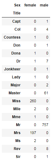
出现次数很少的title归类到'rare',并统计title与生还概率相关性:
full['Title'] = full['Title'].replace(['Capt','Col','Countess','Don','Dona','Dr','Jonkheer','Lady','Major','Mlle','Mme','Ms','Rev','Sir'], 'Rare')
full[['Title', 'Survived']].groupby(['Title'], as_index=False).mean().sort_values(by='Survived', ascending=False)
title与生还概率存在明显的相关关系。
2.2 缺失值填充
full.drop(['Cabin', 'Ticket'], axis=1, inplace=True)
full['Age'] = full['Age'].fillna(full['Age'].mean())
full['Fare'] = full['Fare'].fillna(full['Fare'].mean())
full['Embarked'] = full['Embarked'].fillna('S')
2.3 类别变量转化为数值型
full['Title'] = full['Title'].map({"Mr": 1, "Miss": 2, "Mrs": 3, "Master": 4, "Rare": 5}).astype(int)
full['Sex'] = full['Sex'].map({'female':1, 'male':0}).astype(int)
full['Embarked'] = full['Embarked'].map({'S': 0, 'Q': 1,'C': 2}).astype(int)
2.4 连续变量转化为离散型
年龄等距分箱
full['AgeBand'] = pd.cut(full['Age'], 5)
full[['AgeBand', 'Survived']].groupby(['AgeBand'], as_index=False).mean().sort_values(by='AgeBand', ascending=True)

full.loc[full['Age'] <= 16, 'Age_discrete'] = 0
full.loc[(full['Age'] > 16) & (full['Age'] <= 32), 'Age_discrete'] = 1
full.loc[(full['Age'] > 32) & (full['Age'] <= 48), 'Age_discrete'] = 2
full.loc[(full['Age'] > 48) & (full['Age'] <= 64), 'Age_discrete'] = 3
full.loc[full['Age'] > 64, 'Age_discrete'] = 4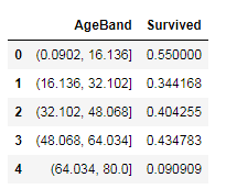
票价等频分箱
full['FareBand'] = pd.qcut(full['Fare'],4)
full[['FareBand', 'Survived']].groupby(['FareBand'], as_index=False).mean().sort_values(by='FareBand', ascending=True)

full.loc[full['Fare'] <= 7.896, 'Fare_discrete'] = 0
full.loc[(full['Fare'] > 7.896) & (full['Fare'] <= 14.454), 'Fare_discrete'] = 1
full.loc[(full['Fare'] > 14.454) & (full['Fare'] <= 31.275), 'Fare_discrete'] = 2
full.loc[(full['Fare'] > 31.275), 'Fare_discrete'] = 3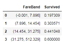
2.5 组合特征变量
考虑所有家人,构建衍生变量:家庭成员数目和是否单独一人
full['FamilySize'] = full['SibSp'] + full['Parch'] + 1
display.display(full[['FamilySize', 'Survived']].groupby(['FamilySize'], as_index=False).mean().sort_values(by='Survived', ascending=False))

full['IsAlone'] = 0
full.loc[full['FamilySize'] == 1, 'IsAlone'] = 1
display.display(full[['IsAlone','Survived']].groupby(['IsAlone'], as_index=False).mean())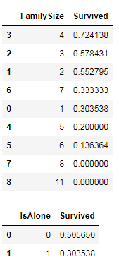
考虑年龄和船舱等级的组合特征:
full['Age*Class'] = full.Age_discrete * full.Pclass
full[['Age*Class', 'Survived']].groupby(['Age*Class'], as_index=False).mean().sort_values(by='Survived', ascending=False)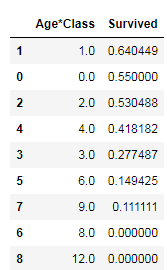
考虑票价和登船地点的组合特征:
full['Fare*Embarked'] = full.Fare_discrete * full.Embarked
full[['Fare*Embarked', 'Survived']].groupby(['Fare*Embarked'], as_index=False).mean().sort_values(by='Survived', ascending=False)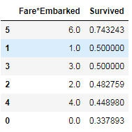
三、模型构建
1、rf模型
#特征选择
full_features = full.loc[:,['Sex','Pclass','Embarked', 'Age', 'Fare', 'Age_discrete', 'Fare_discrete','Parch', 'SibSp', 'FamilySize', 'IsAlone', 'Title', 'Age*Class','Fare*Embarked']]
source_x = full_features.loc[0:890,:]
source_y = full.loc[0:890, 'Survived']
pred_x = full_features.loc[891:,:]

#模型构建
rf = RandomForestClassifier(n_estimators=200, max_depth=7)
rf.fit(source_x,source_y)
pred_y = rf.predict(pred_x)
pred_y = pred_y.astype(int)
display.display(rf.feature_importances_)

#预测结果提交
passenger_id = full.loc[891:, 'PassengerId']
predDF = pd.DataFrame({'PassengerId':passenger_id, 'Survived':pred_y})
display.display(predDF.head())
predDF.to_csv("../rf-submission_14_200_7.csv", index=False)
线上准确率:

参考资料:
https://www.kaggle.com/c/titanic#tutorials
https://www.kaggle.com/startupsci/titanic-data-science-solutions