综述
“以古为镜,可以知兴替;以人为镜,可以明得失。”
本文采用编译器:jupyter
首先提出一个关于分类准确度的问题:
一个癌症预测系统,输入体检信息就可以判断病人是否患有癌症。
如果这个系统的预测准确度为99.9%,这个系统是好是坏?
虽然99.9%的概率看上去比较大,但如果癌症产生的概率只有0.1%的话,我们辛辛苦苦做出来的系统和一个预测所有人都是健康的系统的性能完全相同;如果癌症产生的概率只有0.01%,甚至还不如“傻瓜式”的系统。
所以对于极度偏斜(Skewed Data)的数据,只是用分类准确度是远远不够的,我们需要使用新的分析工具混淆矩阵来做进一步的分析,如下。
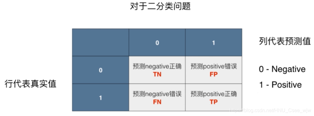
对此,引入精准率和召回率两个概念
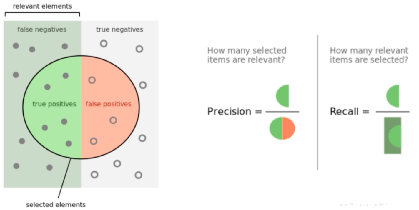
精准率:预测为1且预测正确的概率

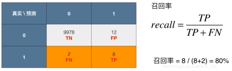
召回率:真实发生了且预测正确的概率
进一步理解:
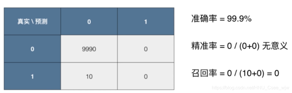
然而有时精准率与召回率也无意义,虽然这种情况发生的概率极小。
01 实现混淆矩阵,精准率和召回率
import numpy as np
from sklearn import datasets
digits = datasets.load_digits()
X = digits.data
y = digits.target.copy()
# 手动使数据变得偏斜
y[digits.target==9] = 1
y[digits.target!=9] = 0
from sklearn.model_selection import train_test_split
X_train, X_test, y_train, y_test = train_test_split(X, y, random_state=666)
from sklearn.linear_model import LogisticRegression
log_reg = LogisticRegression()
log_reg.fit(X_train, y_train)
log_reg.score(X_test, y_test)
# Out[4]:
# 0.97555555555555551
y_log_predict = log_reg.predict(X_test)
def TN(y_true, y_predict):
assert len(y_true) == len(y_predict)
return np.sum((y_true == 0) & (y_predict == 0))
TN(y_test, y_log_predict)
# Out[6]:
# 403
def FP(y_true, y_predict):
assert len(y_true) == len(y_predict)
return np.sum((y_true == 0) & (y_predict == 1))
FP(y_test, y_log_predict)
# Out[7]:
# 2
def FN(y_true, y_predict):
assert len(y_true) == len(y_predict)
return np.sum((y_true == 1) & (y_predict == 0))
FN(y_test, y_log_predict)
# Out[8]:
# 9
def TP(y_true, y_predict):
assert len(y_true) == len(y_predict)
return np.sum((y_true == 1) & (y_predict == 1))
TP(y_test, y_log_predict)
# Out[9]:
# 36
def confusion_matrix(y_true, y_predict):
return np.array([
[TN(y_test, y_log_predict),FP(y_test, y_log_predict)],
[FN(y_test, y_log_predict),TP(y_test, y_log_predict)]
])
confusion_matrix(y_test, y_log_predict)
"""
Out[10]:
array([[403, 2],
[ 9, 36]])
"""
def precision_score(y_true, y_predict):
tp = TP(y_true, y_predict)
fp = FP(y_true, y_predict)
try:
return tp / (tp + fp)
except:
return 0.0
precision_score(y_test, y_log_predict)
# Out[11]:
# 0.94736842105263153
def recall_score(y_true, y_predict):
tp = TP(y_true, y_predict)
fn = FN(y_true, y_predict)
try:
return tp / (tp + fn)
except:
return 0.0
recall_score(y_test, y_log_predict)
# Out[13]:
# 0.80000000000000004scikit-learn中的混淆矩阵,精准率和召回率
from sklearn.metrics import confusion_matrix
confusion_matrix(y_test, y_log_predict)
"""
Out[15]:
array([[403, 2],
[ 9, 36]])
"""
from sklearn.metrics import precision_score
precision_score(y_test, y_log_predict)
# Out[16]:
# 0.94736842105263153
from sklearn.metrics import recall_score
recall_score(y_test, y_log_predict)
# Out[17]:
# 0.80000000000000004有时候我们注重精准率,如股票预测
预测股票上涨的情况下,实际股票是涨的概率越大越好;而对于前提是股票已经上涨的召回率来看,它的大小不是那么重要。
有时候我们注重召回率,如股票预测
在病人已经得病的前提下,预测为Positive的概率应当越大越好;而对于前提是预测为Positive的精准率来看,则没那么重要,无非是需要病人多做一些检查罢了。
有时,我们想要同时兼顾精准率与召回率,对此定义了F1 Score
F1 Score是precision和recall的调和平均值
02 F1 Score
import numpy as np
def f1_score(precision, recall):
try:
return 2 * precision * recall / (precision + recall)
except:
# 防止分母为0
return 0.0
precision = 0.5
recall = 0.5
f1_score(precision, recall)
# Out[3]:
# 0.5
precision = 0.1
recall = 0.9
f1_score(precision, recall)
# Out[5]:
# 0.18000000000000002
precision = 0.0
recall = 1.0
f1_score(precision, recall)
# Out[6]:
# 0.0
from sklearn import datasets
digits = datasets.load_digits()
X = digits.data
y = digits.target.copy()
# 手动使数据变得偏斜
y[digits.target==9] = 1
y[digits.target!=9] = 0
from sklearn.model_selection import train_test_split
X_train, X_test, y_train, y_test = train_test_split(X, y, random_state=666)
from sklearn.linear_model import LogisticRegression
log_reg = LogisticRegression()
log_reg.fit(X_train, y_train)
log_reg.score(X_test, y_test)
# Out[9]:
# 0.97555555555555551
y_predict = log_reg.predict(X_test)
from sklearn.metrics import confusion_matrix
confusion_matrix(y_test, y_predict)
"""
Out[11]:
array([[403, 2],
[ 9, 36]])
"""
from sklearn.metrics import precision_score
precision_score(y_test, y_predict)
# Out[12]:
# 0.94736842105263153
from sklearn.metrics import recall_score
recall_score(y_test, y_predict)
# Out[13]:
# 0.80000000000000004
from sklearn.metrics import f1_score
f1_score(y_test, y_predict)
# Out[14]:
# 0.86746987951807231Precision-Recall二者通常是互相矛盾的,我们需要找到它的平衡:
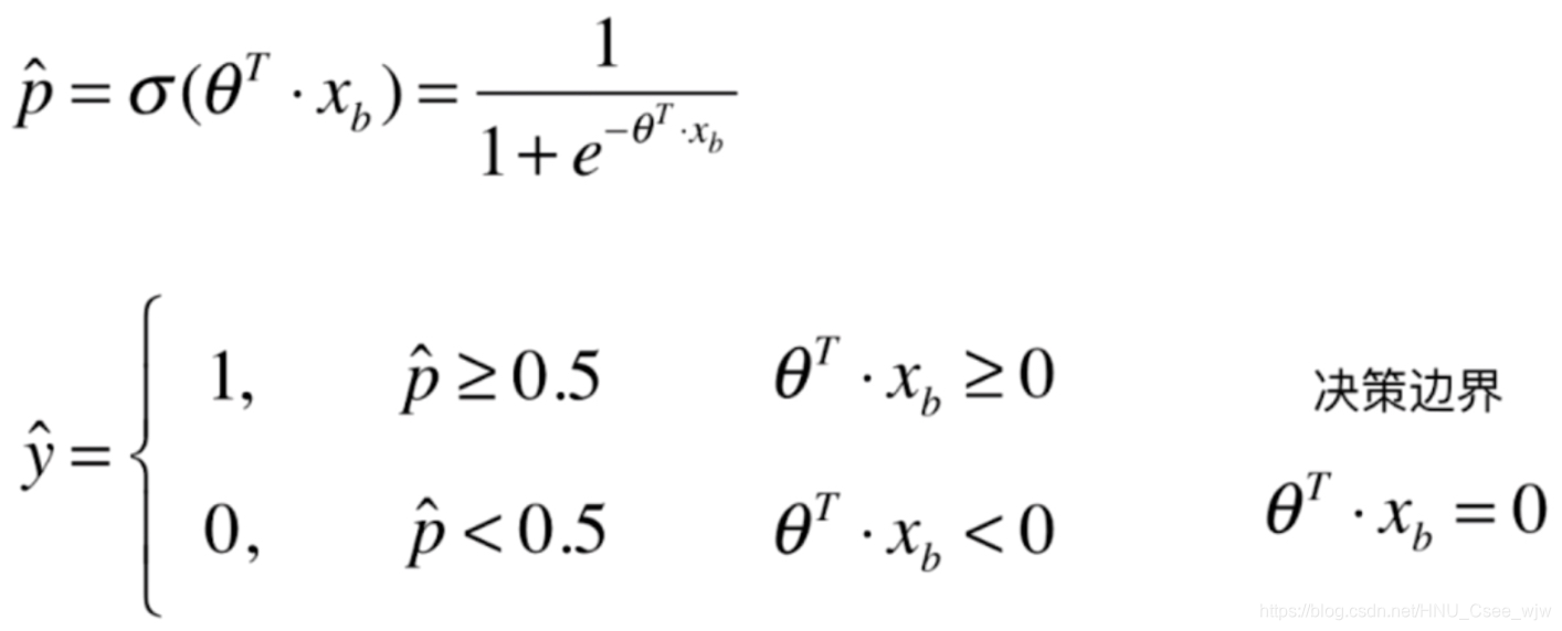
为了方便绘图,我们可以令逻辑回归中的决策边界右边的值等于一个常数,阈值取值不同召回率与精准率也不同,如图。
![]()
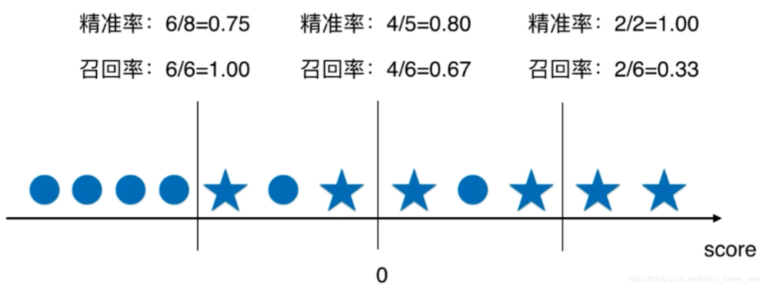
通俗点说,如果想要提高精准率则机器需要在特别有把握(概率很大)的情况下判断为正,使得有一部分为正的样本因为概率不够大而落入判断为负的区域,召回率下降;
如果想要提高召回率,则机器需要降低判断的标准,使得概率不是很大的样本也要被判断为正,相应的也降低了精准率。
03 精准率和召回率的平衡
import numpy as np
import matplotlib.pyplot as plt
from sklearn import datasets
digits = datasets.load_digits()
X = digits.data
y = digits.target.copy()
# 手动产生有偏数据集
y[digits.target==9] = 1
y[digits.target!=9] = 0
from sklearn.model_selection import train_test_split
X_train, X_test, y_train, y_test = train_test_split(X, y, random_state=666)
from sklearn.linear_model import LogisticRegression
log_reg = LogisticRegression()
log_reg.fit(X_train, y_train)
y_predict = log_reg.predict(X_test)
from sklearn.metrics import f1_score
f1_score(y_test, y_predict)
# Out[6]:
# 0.86746987951807231
from sklearn.metrics import confusion_matrix
confusion_matrix(y_test, y_predict)
"""
Out[7]:
array([[403, 2],
[ 9, 36]])
"""
# 查看X_test每个数据对应的Score值,即“概率”
log_reg.decision_function(X_test)
"""
Out[8]:
array([-22.0570091 , -33.02945537, -16.21336318, -80.37913541,
-48.25120952, -24.54005626, -44.39160994, -25.04295391,
-0.97827422, -19.71741808, -66.2513508 , -51.09606598,
-31.49350877, -46.05329887, -38.67883906, -29.80470208,
-37.58854929, -82.57573674, -37.81899199, -11.01168647,
......
-68.31025868, -6.2593453 , -25.83997855, -38.00873296,
-27.90916079, -15.44714767, -27.45898314, -19.59776151,
12.33461808, -23.03864955, -35.94464178, -30.0283688 ,
-14.98142887, -24.83600055, -16.93960455, -19.46791858,
-26.98681137, -32.38775186, -28.96086511, -67.25181176,
-46.49541088, -16.11287354])
"""
log_reg.decision_function(X_test)[:10]
"""
Out[9]:
array([-22.0570091 , -33.02945537, -16.21336318, -80.37913541,
-48.25120952, -24.54005626, -44.39160994, -25.04295391,
-0.97827422, -19.71741808])
"""
# 查看根据“概率”的判决结果
log_reg.predict(X_test)[:10]
# Out[10]:
# array([0, 0, 0, 0, 0, 0, 0, 0, 0, 0])
decision_scores = log_reg.decision_function(X_test)
np.min(decision_scores)
# Out[12]:
# -85.686140912160724
np.max(decision_scores)
# Out[13]:
# 19.889625923668461
# 将决策阈值设置为5,召回率小,精准率大
y_predict_2 = np.array(decision_scores >= 5, dtype='int')
confusion_matrix(y_test, y_predict_2)
"""
Out[15]:
array([[404, 1],
[ 21, 24]])
"""
from sklearn.metrics import precision_score
precision_score(y_test, y_predict_2)
# Out[17]:
# 0.95999999999999996
from sklearn.metrics import recall_score
recall_score(y_test, y_predict_2)
# Out[18]:
# 0.53333333333333333
# 将决策阈值设置为-5,召回率大,精准率小
y_predict_3 = np.array(decision_scores >= -5, dtype='int')
confusion_matrix(y_test, y_predict_3)
"""
Out[20]:
array([[390, 15],
[ 5, 40]])
"""
precision_score(y_test, y_predict_3)
# Out[21]:
# 0.72727272727272729
recall_score(y_test, y_predict_3)
# Out[22]:
# 0.8888888888888888404 可视化精准率和召回率的平衡
import numpy as np
import matplotlib.pyplot as plt
from sklearn import datasets
digits = datasets.load_digits()
X = digits.data
y = digits.target.copy()
# 手动产生有偏数据集
y[digits.target==9] = 1
y[digits.target!=9] = 0
from sklearn.model_selection import train_test_split
X_train, X_test, y_train, y_test = train_test_split(X, y, random_state=666)
from sklearn.linear_model import LogisticRegression
log_reg = LogisticRegression()
log_reg.fit(X_train, y_train)
decision_scores = log_reg.decision_function(X_test)
from sklearn.metrics import precision_score
from sklearn.metrics import recall_score
precisions = []
recalls = []
# 在决策score最小与最大之间构造数组
thresholds = np.arange(np.min(decision_scores), np.max(decision_scores), 0.1)
for threshold in thresholds:
y_predict = np.array(decision_scores >= threshold, dtype='int')
precisions.append(precision_score(y_test, y_predict))
recalls.append(recall_score(y_test, y_predict))
plt.plot(thresholds, precisions)
plt.plot(thresholds, recalls)
plt.show()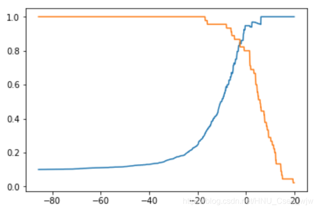
Precision-Recall曲线
plt.plot(precisions, recalls)
plt.show()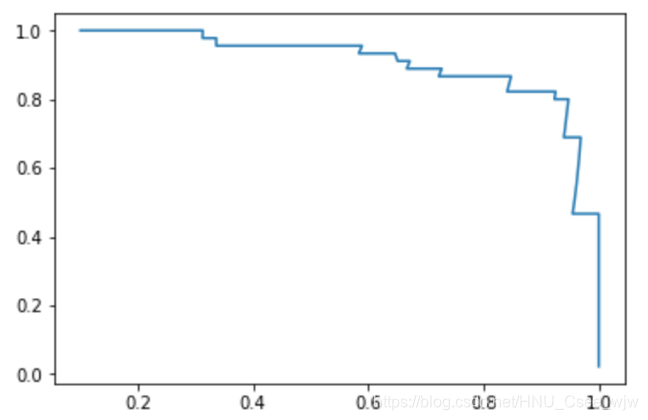
scikit-learn中的Precision-Recall曲线
from sklearn.metrics import precision_recall_curve
precisions, recalls, thresholds = precision_recall_curve(y_test, decision_scores)
precisions.shape # 步长由函数自动给出
# Out[9]:
# (145,)
recalls.shape
# Out[10]:
# (145,)
# 查阅文档可知,最后一个精确率和召回率的值分别为1和0,并且没有对应的threshold值
thresholds.shape
# Out[11]:
# (144,)
# 去除最后一个值以保证维度相同
plt.plot(thresholds, precisions[:-1])
plt.plot(thresholds, recalls[:-1])
plt.show()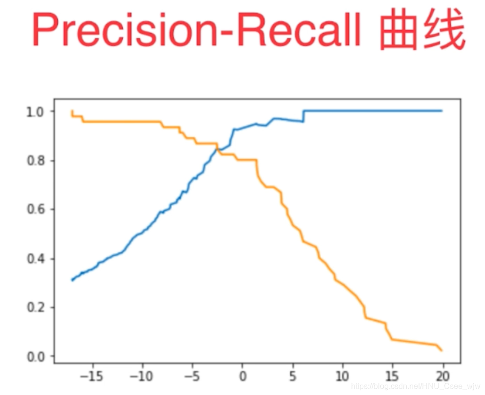
plt.plot(precisions, recalls)
plt.show()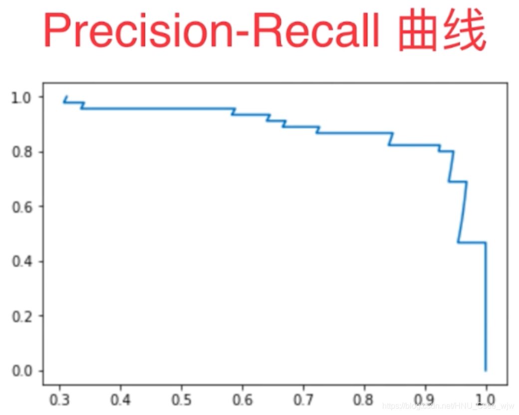
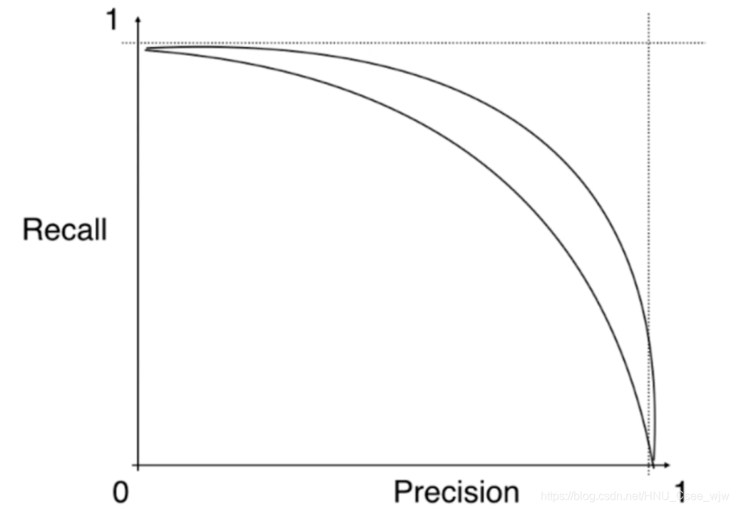
PR曲线越靠外则模型越好
ROC曲线:
Receiver Operation Characteristic Curve,用来描述TPR和FPR之间的关系
TPR:预测为1,且预测对了
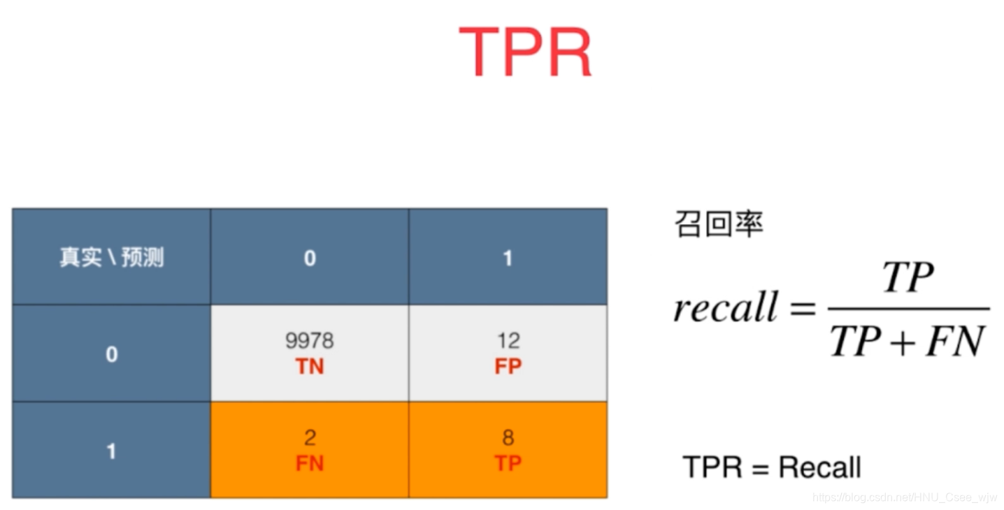
FPR:预测为1,且预测错了
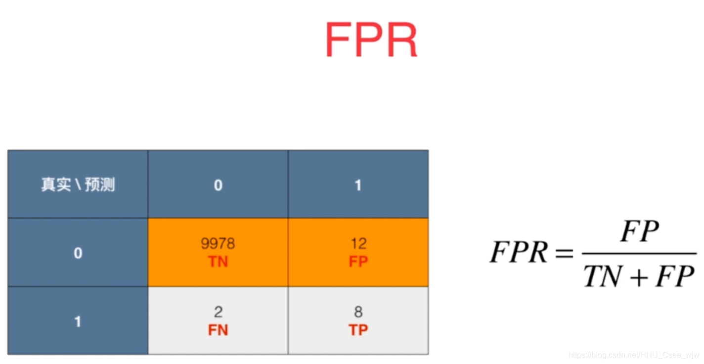
FPR与TPR随着决策阈值的变化而同时增加或减小

05 ROC曲线
import numpy as np
import matplotlib.pyplot as plt
from sklearn import datasets
digits = datasets.load_digits()
X = digits.data
y = digits.target.copy()
# 手动产生有偏数据集
y[digits.target==9] = 1
y[digits.target!=9] = 0
from sklearn.model_selection import train_test_split
X_train, X_test, y_train, y_test = train_test_split(X, y, random_state=666)
from sklearn.linear_model import LogisticRegression
log_reg = LogisticRegression()
log_reg.fit(X_train, y_train)
decision_scores = log_reg.decision_function(X_test)
from playML.metrics import FPR, TPR
fprs = []
tprs = []
thresholds = np.arange(np.min(decision_scores), np.max(decision_scores), 0.1)
for threshold in thresholds:
y_predict = np.array(decision_scores >= threshold, dtype='int')
fprs.append(FPR(y_test, y_predict))
tprs.append(TPR(y_test, y_predict))
plt.plot(fprs, tprs)
plt.show()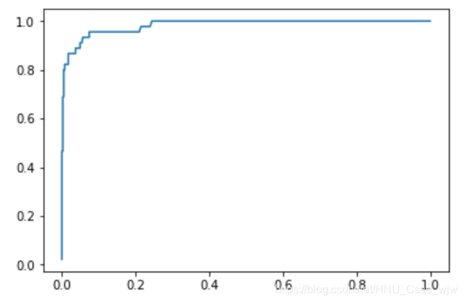
scikit-learn中的ROC
from sklearn.metrics import roc_curve
fprs, tprs, thresholds = roc_curve(y_test, decision_scores)
plt.plot(fprs, tprs)
plt.show()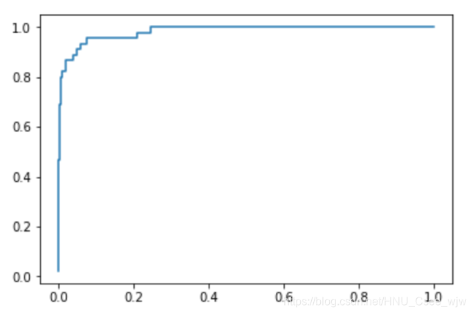
## 求曲线与坐标轴的面积可以作为衡量模型的标准
from sklearn.metrics import roc_auc_score
roc_auc_score(y_test, decision_scores)
# Out[12]:
# 0.98304526748971188
06 多分类问题中的混淆矩阵
import numpy as np
import matplotlib.pyplot as plt
from sklearn import datasets
digits = datasets.load_digits()
X = digits.data
y = digits.target
from sklearn.model_selection import train_test_split
X_train, X_test, y_train, y_test = train_test_split(X, y, test_size=0.8, random_state=666)
from sklearn.linear_model import LogisticRegression
log_reg = LogisticRegression()
log_reg.fit(X_train, y_train)
log_reg.score(X_test, y_test)
# Out[6]:
# 0.93115438108484005
y_predict = log_reg.predict(X_test)
from sklearn.metrics import precision_score
# 计算多分类问题的精准率(参考文档)
precision_score(y_test, y_predict, average='micro')
# Out[10]:
# 0.93115438108484005
from sklearn.metrics import confusion_matrix
# 混淆矩阵对角线即为预测正确的情况
confusion_matrix(y_test, y_predict)
"""
Out[12]:
array([[147, 0, 1, 0, 0, 1, 0, 0, 0, 0],
[ 0, 123, 1, 2, 0, 0, 0, 3, 4, 10],
[ 0, 0, 134, 1, 0, 0, 0, 0, 1, 0],
[ 0, 0, 0, 138, 0, 5, 0, 1, 5, 0],
[ 2, 5, 0, 0, 139, 0, 0, 3, 0, 1],
[ 1, 3, 1, 0, 0, 146, 0, 0, 1, 0],
[ 0, 2, 0, 0, 0, 1, 131, 0, 2, 0],
[ 0, 0, 0, 1, 0, 0, 0, 132, 1, 2],
[ 1, 9, 2, 3, 2, 4, 0, 0, 115, 4],
[ 0, 1, 0, 5, 0, 3, 0, 2, 2, 134]])
"""
cfm = confusion_matrix(y_test, y_predict)
plt.matshow(cfm, cmap=plt.cm.gray) # 颜色映射
plt.show()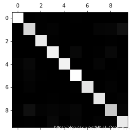
# 计算每一行的和
row_sums = np.sum(cfm, axis=1)
err_matrix = cfm / row_sums
# 由于不关注分类正确的情况,所以将对角线的数字全部填充为0
np.fill_diagonal(err_matrix, 0)
err_matrix
"""
Out[15]:
array([[ 0.        ,  0.        ,  0.00735294,  0.        ,  0.        ,
         0.00657895,  0.        ,  0.        ,  0.        ,  0.        ],
       [ 0.        ,  0.        ,  0.00735294,  0.01342282,  0.        ,
         0.        ,  0.        ,  0.02205882,  0.02857143,  0.06802721],
       [ 0.        ,  0.        ,  0.        ,  0.00671141,  0.        ,
         0.        ,  0.        ,  0.        ,  0.00714286,  0.        ],
       [ 0.        ,  0.        ,  0.        ,  0.        ,  0.        ,
         0.03289474,  0.        ,  0.00735294,  0.03571429,  0.        ],
       [ 0.01342282,  0.03496503,  0.        ,  0.        ,  0.        ,
         0.        ,  0.        ,  0.02205882,  0.        ,  0.00680272],
       [ 0.00671141,  0.02097902,  0.00735294,  0.        ,  0.        ,
         0.        ,  0.        ,  0.        ,  0.00714286,  0.        ],
       [ 0.        ,  0.01398601,  0.        ,  0.        ,  0.        ,
         0.00657895,  0.        ,  0.        ,  0.01428571,  0.        ],
       [ 0.        ,  0.        ,  0.        ,  0.00671141,  0.        ,
         0.        ,  0.        ,  0.        ,  0.00714286,  0.01360544],
       [ 0.00671141,  0.06293706,  0.01470588,  0.02013423,  0.01333333,
         0.02631579,  0.        ,  0.        ,  0.        ,  0.02721088],
       [ 0.        ,  0.00699301,  0.        ,  0.03355705,  0.        ,
         0.01973684,  0.        ,  0.01470588,  0.01428571,  0.        ]])
"""
cfm = confusion_matrix(y_test, y_predict)
plt.matshow(err_matrix, cmap=plt.cm.gray) # 颜色映射
plt.show()
# 颜色越白的点表示错误越大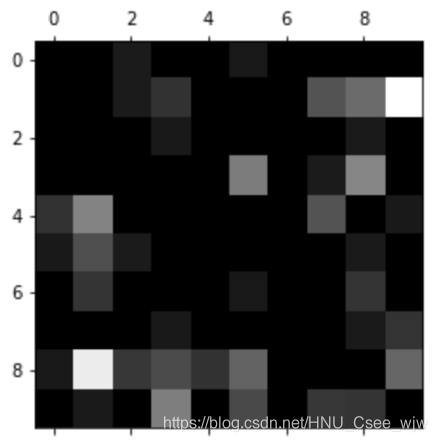
最后,如果有什么疑问,欢迎和我微信交流。
