目录
2. HAN的原理(Hierarchical Attention Networks)
1. 基本的Attention原理
1.1 Attention背景及作用
深度学习中的注意力机制从本质上讲和人类的选择性视觉注意力机制类似,核心目标也是从众多信息中选择出对当前任务目标更关键的信息。
Attention的出现就是为了两个目的:1. 减小处理高维输入数据的计算负担,通过结构化的选取输入的子集,降低数据维度。2. “去伪存真”,让任务处理系统更专注于找到输入数据中显著的与当前输出相关的有用信息,从而提高输出的质量。Attention模型的最终目的是帮助类似编解码器这样的框架,更好的学到多种内容模态之间的相互关系,从而更好的表示这些信息,克服其无法解释从而很难设计的缺陷。从上述的研究问题可以发现,Attention机制非常适合于推理多种不同模态数据之间的相互映射关系,这种关系很难解释,很隐蔽也很复杂,这正是Attention的优势—不需要监督信号,对于上述这种认知先验极少的问题,显得极为有效。
1.2 为什么要引入Attention机制
根据通用近似定理,前馈网络和循环网络都有很强的能力。但为什么还要引入注意力机制呢?
- 计算能力的限制:当要记住很多“信息“,模型就要变得更复杂,然而目前计算能力依然是限制神经网络发展的瓶颈。
- 优化算法的限制:虽然局部连接、权重共享以及pooling等优化操作可以让神经网络变得简单一些,有效缓解模型复杂度和表达能力之间的矛盾;但是,如循环神经网络中的长距离以来问题,信息“记忆”能力并不高。
可以借助人脑处理信息过载的方式,例如Attention机制可以提高神经网络处理信息的能力。
1.3 Attention机制分类
当用神经网络来处理大量的输入信息时,也可以借鉴人脑的注意力机制,只 选择一些关键的信息输入进行处理,来提高神经网络的效率。按照认知神经学中的注意力,可以总体上分为两类:
- 聚焦式(focus)注意力:自上而下的有意识的注意力,主动注意——是指有预定目的、依赖任务的、主动有意识地聚焦于某一对象的注意力;
- 显著性(saliency-based)注意力:自下而上的有意识的注意力,被动注意——基于显著性的注意力是由外界刺激驱动的注意,不需要主动干预,也和任务无关;可以将max-pooling和门控(gating)机制来近似地看作是自下而上的基于显著性的注意力机制。
在人工神经网络中,注意力机制一般就特指聚焦式注意力。
1.4 Attention机制的计算流程

Attention机制的实质其实就是一个寻址(addressing)的过程,如上图所示:给定一个和任务相关的查询Query向量 q,通过计算与Key的注意力分布并附加在Value上,从而计算Attention Value,这个过程实际上是Attention机制缓解神经网络模型复杂度的体现:不需要将所有的N个输入信息都输入到神经网络进行计算,只需要从X中选择一些和任务相关的信息输入给神经网络。
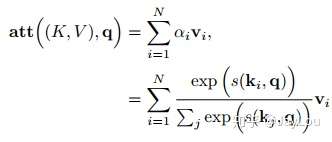
注意力机制可以分为三步:一是信息输入;二是计算注意力分布α;三是根据注意力分布α 来计算输入信息的加权平均。
step1-信息输入:用X = [x1, · · · , xN ]表示N 个输入信息;
step2-注意力分布计算:令Key=Value=X,则可以给出注意力分布
我们将 称之为注意力分布(概率分布),
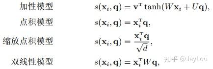
为注意力打分机制,有几种打分机制:
step3-信息加权平均:注意力分布 可以解释为在上下文查询q时,第i个信息受关注的程度,采用一种“软性”的信息选择机制对输入信息X进行编码为:
这种编码方式为软性注意力机制(soft Attention),软性注意力机制有两种:普通模式(Key=Value=X)和键值对模式(Key!=Value)。
1.5 Attention机制的变种
与普通的Attention机制(上图左)相比,Attention机制有哪些变种呢?
- 变种1-硬性注意力:之前提到的注意力是软性注意力,其选择的信息是所有输入信息在注意力 分布下的期望。还有一种注意力是只关注到某一个位置上的信息,叫做硬性注意力(hard attention)。硬性注意力有两种实现方式:(1)一种是选取最高概率的输入信息;(2)另一种硬性注意力可以通过在注意力分布式上随机采样的方式实现。硬性注意力模型的缺点:
硬性注意力的一个缺点是基于最大采样或随机采样的方式来选择信息。因此最终的损失函数与注意力分布之间的函数关系不可导,因此无法使用在反向传播算法进行训练。为了使用反向传播算法,一般使用软性注意力来代替硬性注意力。硬性注意力需要通过强化学习来进行训练。—— 《神经网络与深度学习》
- 变种2-键值对注意力:即上图右边的键值对模式,此时Key!=Value,注意力函数变为:

变种3-多头注意力:多头注意力(multi-head attention)是利用多个查询Q = [q1, · · · , qM],来平行地计算从输入信息中选取多个信息。每个注意力关注输入信息的不同部分,然后再进行拼接:

2. HAN的原理(Hierarchical Attention Networks)
HAN模型就是分层次的利用注意力机制来构建文本向量表示的方法。
文本由句子构成,句子由词构成,HAN模型对应这个结构分层的来构建文本向量表达;
文本中不同句子对文本的主旨影响程度不同,一个句子中不同的词语对句子主旨的影响程度也不同,因此HAN在词语层面和句子层面分别添加了注意力机制;
分层的注意力机制还有一个好处,可以直观的看出用这个模型构建文本表示时各个句子和单词的重要程度,增强了可解释性;
模型结构:

3. 利用Attention模型进行文本分类
参考:Tensorflow implementation of attention mechanism for text classification tasks
utils.py
from __future__ import print_function

import numpy as np


def zero_pad(X, seq_len):
    return np.array([x[:seq_len - 1] + [0] * max(seq_len - len(x), 1) for x in X])


def get_vocabulary_size(X):
    return max([max(x) for x in X]) + 1  # plus the 0th word


def fit_in_vocabulary(X, voc_size):
    return [[w for w in x if w < voc_size] for x in X]


def batch_generator(X, y, batch_size):
    """Primitive batch generator
    """
    size = X.shape[0]
    X_copy = X.copy()
    y_copy = y.copy()
    indices = np.arange(size)
    np.random.shuffle(indices)
    X_copy = X_copy[indices]
    y_copy = y_copy[indices]
    i = 0
    while True:
        if i + batch_size <= size:
            yield X_copy[i:i + batch_size], y_copy[i:i + batch_size]
            i += batch_size
        else:
            i = 0
            indices = np.arange(size)
            np.random.shuffle(indices)
            X_copy = X_copy[indices]
            y_copy = y_copy[indices]
            continue


if __name__ == "__main__":
    # Test batch generator
    gen = batch_generator(np.array(['a', 'b', 'c', 'd']), np.array([1, 2, 3, 4]), 2)
    for _ in range(8):
        xx, yy = next(gen)
        print(xx, yy)
attention.py
import tensorflow as tf


def attention(inputs, attention_size, time_major=False, return_alphas=False):


    if isinstance(inputs, tuple):
        # In case of Bi-RNN, concatenate the forward and the backward RNN outputs.
        inputs = tf.concat(inputs, 2)

    if time_major:
        # (T,B,D) => (B,T,D)
        inputs = tf.array_ops.transpose(inputs, [1, 0, 2])

    hidden_size = inputs.shape[2].value  # D value - hidden size of the RNN layer

    # Trainable parameters
    w_omega = tf.Variable(tf.random_normal([hidden_size, attention_size], stddev=0.1))
    b_omega = tf.Variable(tf.random_normal([attention_size], stddev=0.1))
    u_omega = tf.Variable(tf.random_normal([attention_size], stddev=0.1))

    with tf.name_scope('v'):
        # Applying fully connected layer with non-linear activation to each of the B*T timestamps;
        #  the shape of `v` is (B,T,D)*(D,A)=(B,T,A), where A=attention_size
        v = tf.tanh(tf.tensordot(inputs, w_omega, axes=1) + b_omega)

    # For each of the timestamps its vector of size A from `v` is reduced with `u` vector
    vu = tf.tensordot(v, u_omega, axes=1, name='vu')  # (B,T) shape
    alphas = tf.nn.softmax(vu, name='alphas')         # (B,T) shape

    # Output of (Bi-)RNN is reduced with attention vector; the result has (B,D) shape
    output = tf.reduce_sum(inputs * tf.expand_dims(alphas, -1), 1)

    if not return_alphas:
        return output
    else:
        return output, alphas
train.py
#!/usr/bin/python
"""
Toy example of attention layer use

Train RNN (GRU) on IMDB dataset (binary classification)
Learning and hyper-parameters were not tuned; script serves as an example
"""
from __future__ import print_function, division

import numpy as np
import tensorflow as tf
from keras.datasets import imdb
from tensorflow.contrib.rnn import GRUCell
from tensorflow.python.ops.rnn import bidirectional_dynamic_rnn as bi_rnn
from tqdm import tqdm

from attention import attention
from utils import get_vocabulary_size, fit_in_vocabulary, zero_pad, batch_generator

NUM_WORDS = 10000
INDEX_FROM = 3
SEQUENCE_LENGTH = 250
EMBEDDING_DIM = 100
HIDDEN_SIZE = 150
ATTENTION_SIZE = 50
KEEP_PROB = 0.8
BATCH_SIZE = 256
NUM_EPOCHS = 3  # Model easily overfits without pre-trained words embeddings, that's why train for a few epochs
DELTA = 0.5
MODEL_PATH = './model'

# Load the data set
(X_train, y_train), (X_test, y_test) = imdb.load_data(num_words=NUM_WORDS, index_from=INDEX_FROM)

# Sequences pre-processing
vocabulary_size = get_vocabulary_size(X_train)
X_test = fit_in_vocabulary(X_test, vocabulary_size)
X_train = zero_pad(X_train, SEQUENCE_LENGTH)
X_test = zero_pad(X_test, SEQUENCE_LENGTH)

# Different placeholders
with tf.name_scope('Inputs'):
    batch_ph = tf.placeholder(tf.int32, [None, SEQUENCE_LENGTH], name='batch_ph')
    target_ph = tf.placeholder(tf.float32, [None], name='target_ph')
    seq_len_ph = tf.placeholder(tf.int32, [None], name='seq_len_ph')
    keep_prob_ph = tf.placeholder(tf.float32, name='keep_prob_ph')

# Embedding layer
with tf.name_scope('Embedding_layer'):
    embeddings_var = tf.Variable(tf.random_uniform([vocabulary_size, EMBEDDING_DIM], -1.0, 1.0), trainable=True)
    tf.summary.histogram('embeddings_var', embeddings_var)
    batch_embedded = tf.nn.embedding_lookup(embeddings_var, batch_ph)

# (Bi-)RNN layer(-s)
rnn_outputs, _ = bi_rnn(GRUCell(HIDDEN_SIZE), GRUCell(HIDDEN_SIZE),
                        inputs=batch_embedded, sequence_length=seq_len_ph, dtype=tf.float32)
tf.summary.histogram('RNN_outputs', rnn_outputs)

# Attention layer
with tf.name_scope('Attention_layer'):
    attention_output, alphas = attention(rnn_outputs, ATTENTION_SIZE, return_alphas=True)
    tf.summary.histogram('alphas', alphas)

# Dropout
drop = tf.nn.dropout(attention_output, keep_prob_ph)

# Fully connected layer
with tf.name_scope('Fully_connected_layer'):
    W = tf.Variable(tf.truncated_normal([HIDDEN_SIZE * 2, 1], stddev=0.1))  # Hidden size is multiplied by 2 for Bi-RNN
    b = tf.Variable(tf.constant(0., shape=[1]))
    y_hat = tf.nn.xw_plus_b(drop, W, b)
    y_hat = tf.squeeze(y_hat)
    tf.summary.histogram('W', W)

with tf.name_scope('Metrics'):
    # Cross-entropy loss and optimizer initialization
    loss = tf.reduce_mean(tf.nn.sigmoid_cross_entropy_with_logits(logits=y_hat, labels=target_ph))
    tf.summary.scalar('loss', loss)
    optimizer = tf.train.AdamOptimizer(learning_rate=1e-3).minimize(loss)

    # Accuracy metric
    accuracy = tf.reduce_mean(tf.cast(tf.equal(tf.round(tf.sigmoid(y_hat)), target_ph), tf.float32))
    tf.summary.scalar('accuracy', accuracy)

merged = tf.summary.merge_all()

# Batch generators
train_batch_generator = batch_generator(X_train, y_train, BATCH_SIZE)
test_batch_generator = batch_generator(X_test, y_test, BATCH_SIZE)

train_writer = tf.summary.FileWriter('./logdir/train', accuracy.graph)
test_writer = tf.summary.FileWriter('./logdir/test', accuracy.graph)

session_conf = tf.ConfigProto(gpu_options=tf.GPUOptions(allow_growth=True))

saver = tf.train.Saver()

if __name__ == "__main__":
    with tf.Session(config=session_conf) as sess:
        sess.run(tf.global_variables_initializer())
        print("Start learning...")
        for epoch in range(NUM_EPOCHS):
            loss_train = 0
            loss_test = 0
            accuracy_train = 0
            accuracy_test = 0

            print("epoch: {}\t".format(epoch), end="")

            # Training
            num_batches = X_train.shape[0] // BATCH_SIZE
            for b in tqdm(range(num_batches)):
                x_batch, y_batch = next(train_batch_generator)
                seq_len = np.array([list(x).index(0) + 1 for x in x_batch])  # actual lengths of sequences
                loss_tr, acc, _, summary = sess.run([loss, accuracy, optimizer, merged],
                                                    feed_dict={batch_ph: x_batch,
                                                               target_ph: y_batch,
                                                               seq_len_ph: seq_len,
                                                               keep_prob_ph: KEEP_PROB})
                accuracy_train += acc
                loss_train = loss_tr * DELTA + loss_train * (1 - DELTA)
                train_writer.add_summary(summary, b + num_batches * epoch)
            accuracy_train /= num_batches

            # Testing
            num_batches = X_test.shape[0] // BATCH_SIZE
            for b in tqdm(range(num_batches)):
                x_batch, y_batch = next(test_batch_generator)
                seq_len = np.array([list(x).index(0) + 1 for x in x_batch])  # actual lengths of sequences
                loss_test_batch, acc, summary = sess.run([loss, accuracy, merged],
                                                         feed_dict={batch_ph: x_batch,
                                                                    target_ph: y_batch,
                                                                    seq_len_ph: seq_len,
                                                                    keep_prob_ph: 1.0})
                accuracy_test += acc
                loss_test += loss_test_batch
                test_writer.add_summary(summary, b + num_batches * epoch)
            accuracy_test /= num_batches
            loss_test /= num_batches

            print("loss: {:.3f}, val_loss: {:.3f}, acc: {:.3f}, val_acc: {:.3f}".format(
                loss_train, loss_test, accuracy_train, accuracy_test
            ))
        train_writer.close()
        test_writer.close()
        saver.save(sess, MODEL_PATH)
        print("Run 'tensorboard --logdir=./logdir' to checkout tensorboard logs.")


参考:https://www.zhihu.com/question/68482809/answer/597944559