Introduction
PyTorch v TensorFlow - 你有多少次在社交媒体上看到这个极化问题? 近年来深度学习的兴起得益于这些框架的普及。 两者都有坚定的支持者,但去年开始出现明显的赢家。
PyTorch是2018年最受欢迎的框架之一。它很快成为学术界和业界研究人员首选的深度学习框架。 在过去几周使用PyTorch之后,我可以确认它是高度灵活的,并且是一个易于使用的深度学习库。
在本文中,我们将探讨PyTorch的全部内容。 但是我们的学习不会停留在理论上 - 我们将通过4种不同的用例进行编码,看看PyTorch的表现如何。 建立深度学习模型从未如此有趣!
Contents
- 什么是PyTorch?
- 使用PyTorch构建神经网络
- 用例1:手写数字分类(数字数据,MLP)
- 用例2:对象图像分类(图像数据,CNN)
- 用例3:情感文本分类(文本数据,RNN)
- 用例4:图像样式转移(转移学习)
What is PyTorch?
让我们了解PyTorch是什么以及为什么它最近变得如此受欢迎,然后再深入实施。
PyTorch是一个基于Python的科学计算软件包,类似于NumPy,但增加了GPU的功能。它也是一个深度学习框架,在实施和构建深度神经网络架构时提供最大的灵活性和速度。
最近,PyTorch 1.0发布,旨在通过解决四大挑战来帮助研究人员:
- 广泛的返工
- 耗时的培训
- Python编程语言缺乏灵活性
- 缓慢放大
从本质上讲,PyTorch有两个主要特征,可以将其与其他深度学习框架区分开来:
- 命令式编程
- 动态计算图形
命令式编程:PyTorch在编写代码的每一行时执行计算。这与Python程序的执行方式非常相似。这个概念称为命令式编程。此功能的最大优点是可以动态调试代码和编程逻辑。
动态计算图形:PyTorch被称为“运行定义”框架,这意味着(运行时)生成计算图形结构(神经网络体系结构)。 该属性的主要优点是它提供了灵活的编程运行时接口,通过连接操作来简化系统的构建和修改。 在PyTorch中,在每个前向传递中定义了新的计算图。 这与使用静态图表示的TensorFlow形成鲜明对比。
PyTorch 1.0附带了一个名为torch.jit的重要功能,这是一个高级编译器,允许用户分离模型和代码。 它还支持自定义硬件(如GPU或TPU)上的高效模型优化。
Building Neural Nets using PyTorch
让我们通过更实用的镜头了解PyTorch。 学习理论很好,但是如果你不把它付诸实践就没有多大用处!
神经网络的PyTorch实现看起来与NumPy实现完全相同。 本节的目的是展示PyTorch和NumPy的等效特性。 为此,我们创建一个简单的三层网络,在输入层有5个节点,隐藏层有3个节点,输出层有1个节点。 我们将仅使用一个训练示例,其中一行具有五个特征和一个目标。
import torch
n_input, n_hidden, n_output = 5, 3, 1
第一步是进行参数初始化。 这里,每层的权重和偏差参数被初始化为张量变量。 张量是PyTorch的基础数据结构,用于构建不同类型的神经网络。 它们可以被认为是数组和矩阵的推广; 换句话说,张量是N维矩阵。
## initialize tensor for inputs, and outputs
x = torch.randn((1, n_input))
y = torch.randn((1, n_output))
## initialize tensor variables for weights
w1 = torch.randn(n_input, n_hidden) # weight for hidden layer
w2 = torch.randn(n_hidden, n_output) # weight for output layer
## initialize tensor variables for bias terms
b1 = torch.randn((1, n_hidden)) # bias for hidden layer
b2 = torch.randn((1, n_output)) # bias for output layer
在参数初始化步骤之后,可以通过四个关键步骤定义和训练神经网络:
- 前向传播
- 损失计算
- 反向传播
- 更新参数
让我们更详细地看一下这些步骤。
前向传播:在此步骤中,使用下面显示的两个步骤计算每一层的激活。 这些激活在从输入层到输出层的正向方向上流动,以便产生最终输出。
- z = weight * input + bias
- a = activation_function (z)
以下代码块显示了我们如何在PyTorch中编写这些步骤。 请注意,大多数函数(如指数和矩阵乘法)与NumPy中的函数类似。
## sigmoid activation function using pytorch
def sigmoid_activation(z):
    return 1 / (1 + torch.exp(-z))
## activation of hidden layer
z1 = torch.mm(x, w1) + b1
a1 = sigmoid_activation(z1)
## activation (output) of final layer
z2 = torch.mm(a1, w2) + b2
output = sigmoid_activation(z2)
损耗计算:在此步骤中,在输出层中计算误差(也称为损耗)。 简单的损失函数可以分辨实际值和预测值之间的差异。 稍后,我们将介绍PyTorch中可用的不同损失函数。
loss = y - output
反向传播:此步骤的目的是通过对偏差和权重进行边际变化来最小化输出层中的误差。 使用误差项的导数计算这些边际变化。
基于链规则的微积分原理,将delta变化反馈到隐藏层,其中进行相应的权重和偏差变化。 这导致重量和偏置的调整,直到误差最小化。
## function to calculate the derivative of activation
def sigmoid_delta(x):
  return x * (1 - x)
## compute derivative of error terms
delta_output = sigmoid_delta(output)
delta_hidden = sigmoid_delta(a1)
## backpass the changes to previous layers
d_outp = loss * delta_output
loss_h = torch.mm(d_outp, w2.t())
d_hidn = loss_h * delta_hidden
更新参数:最后,使用从上述反向传播步骤接收的增量更改来更新权重和偏差。
learning_rate = 0.1
w2 += torch.mm(a1.t(), d_outp) * learning_rate
w1 += torch.mm(x.t(), d_hidn) * learning_rate
b2 += d_outp.sum() * learning_rate
b1 += d_hidn.sum() * learning_rate
最后,当对具有大量训练示例的多个历元执行这些步骤时,损失减少到最小值。 获得最终的权重和偏差值,然后可以将其用于对看不见的数据进行预测。
Use Case 1: Handwritten Digital Classification
在上一节中,我们看到了一个简单的PyTorch用例,用于从头开始编写神经网络。 在本节中,我们将使用PyTorch(nn,autograd,optim,torchvision,torchtext等)中提供的不同实用程序包来构建和训练神经网络。
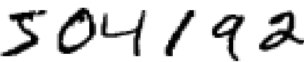
使用这些包可以轻松定义和管理神经网络。 在我们的使用案例中,我们将创建一个多层感知器(MLP)网络,用于构建手写数字分类器。 我们将使用torchvision包中包含的MNIST数据集。
与您正在处理的任何项目一样,第一步是数据预处理。 我们需要将原始数据集转换为张量并在固定范围内对它们进行标准化。 torchvision包提供了一个称为变换的实用程序,可用于将不同的变换组合在一起。
from torchvision import transforms
_tasks = transforms.Compose([
    transforms.ToTensor(),
    transforms.Normalize((0.5, 0.5, 0.5), (0.5, 0.5, 0.5))
    ])
第一个转换将原始数据转换为张量变量,第二个转换使用以下操作执行规范化:
x_normalized = x-mean / std
值0.5和0.5表示3个通道的平均值和标准偏差:红色,绿色和蓝色。
from torchvision.datasets import MNIST
## Load MNIST Dataset and apply transformations
mnist = MNIST("data", download=True, train=True, transform=_tasks)
PyTorch的另一个优秀实用工具是DataLoader迭代器,它提供了使用多处理工作程序并行批处理,混洗和加载数据的能力。 为了评估我们的模型,我们将数据划分为训练和验证集.
from torch.utils.data import DataLoader
from torch.utils.data.sampler import SubsetRandomSampler
## create training and validation split
split = int(0.8 * len(mnist))
index_list = list(range(len(mnist)))
train_idx, valid_idx = index_list[:split], index_list[split:]
## create sampler objects using SubsetRandomSampler
tr_sampler = SubsetRandomSampler(train_idx)
val_sampler = SubsetRandomSampler(valid_idx)
## create iterator objects for train and valid datasets
trainloader = DataLoader(mnist, batch_size=256, sampler=tr_sampler)
validloader = DataLoader(mnist, batch_size=256, sampler=val_sampler)
PyTorch中的神经网络体系结构可以在一个类中定义,该类从名为Module的nn包继承基类的属性。 这种来自nn.Module类的继承允许我们轻松地实现,访问和调用许多方法。 我们可以在类的构造函数中定义所有层,并在forward函数内定义前向传播步骤。
我们将使用以下层配置定义网络:[784,128,10]。 此配置表示输入层中的784个节点(28 * 28像素),隐藏层中的128个节点和输出层中的10个节点。 在forward函数内部,我们将在隐藏层中使用sigmoid激活函数(可以从nn模块访问)。
import torch.nn.functional as F
class Model(nn.Module):
    def __init__(self):
        super().__init__()
        self.hidden = nn.Linear(784, 128)
        self.output = nn.Linear(128, 10)

   def forward(self, x):
        x = self.hidden(x)
        x = F.sigmoid(x)
        x = self.output(x)
        return x
model = Model()
使用nn和optim包定义损失函数和优化器:
from torch import optim
loss_function = nn.CrossEntropyLoss()
optimizer = optim.SGD(model.parameters(), lr=0.01, weight_decay= 1e-6, momentum = 0.9, nesterov = True)
我们现在准备训练模型。 核心步骤将与我们之前看到的相同:前向传播,损失计算,反向传播和更新参数。
for epoch in range(1, 11): ## run the model for 10 epochs
    train_loss, valid_loss = [], []
## training part
    model.train()
    for data, target in trainloader:
        optimizer.zero_grad()
 ## 1. forward propagation
        output = model(data)

        ## 2. loss calculation
        loss = loss_function(output, target)

        ## 3. backward propagation
        loss.backward()

        ## 4. weight optimization
        optimizer.step()

        train_loss.append(loss.item())

    ## evaluation part
    model.eval()
    for data, target in validloader:
        output = model(data)
        loss = loss_function(output, target)
        valid_loss.append(loss.item())
print ("Epoch:", epoch, "Training Loss: ", np.mean(train_loss), "Valid Loss: ", np.mean(valid_loss))
>> Epoch: 1  Training Loss:  0.645777 Valid Loss:  0.344971
>> Epoch: 2  Training Loss:  0.320241 Valid Loss:  0.299313
>> Epoch: 3  Training Loss:  0.278429 Valid Loss:  0.269018
>> Epoch: 4  Training Loss:  0.246289 Valid Loss:  0.237785
>> Epoch: 5  Training Loss:  0.217010 Valid Loss:  0.217133
>> Epoch: 6  Training Loss:  0.193017 Valid Loss:  0.206074
>> Epoch: 7  Training Loss:  0.174385 Valid Loss:  0.180163
>> Epoch: 8  Training Loss:  0.157574 Valid Loss:  0.170064
>> Epoch: 9  Training Loss:  0.144316 Valid Loss:  0.162660
>> Epoch: 10 Training Loss:  0.133053 Valid Loss:  0.152957
Once the model is trained, make the predictions on the validation data.
## dataloader for validation dataset
dataiter = iter(validloader)
data, labels = dataiter.next()
output = model(data)
_, preds_tensor = torch.max(output, 1)
preds = np.squeeze(preds_tensor.numpy())
print ("Actual:", labels[:10])
print ("Predicted:", preds[:10])
>>> Actual: [0 1 1 1 2 2 8 8 2 8]
>>> Predicted: [0 1 1 1 2 2 8 8 2 8]
Use Case 2: Object Image Classification
让我们把事情提升一个档次。
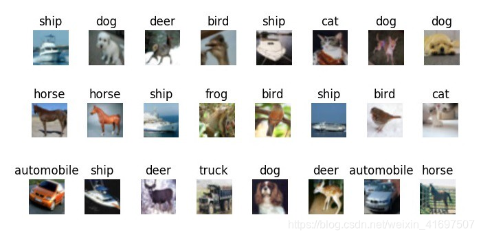
在这个用例中,我们将在PyTorch中创建卷积神经网络(CNN)架构。 我们将使用流行的CIFAR-10数据集执行对象图像分类。 该数据集也包含在torchvision软件包中。 除了在网络中引入附加层之外,定义和训练模型的整个过程将与先前的用例保持相同。
让我们加载并转换数据集:
## load the dataset
from torchvision.datasets import CIFAR10
cifar = CIFAR10('data', train=True, download=True, transform=_tasks)
## create training and validation split
split = int(0.8 * len(cifar))
index_list = list(range(len(cifar)))
train_idx, valid_idx = index_list[:split], index_list[split:]
## create training and validation sampler objects
tr_sampler = SubsetRandomSampler(train_idx)
val_sampler = SubsetRandomSampler(valid_idx)
## create iterator objects for train and valid datasets
trainloader = DataLoader(cifar, batch_size=256, sampler=tr_sampler)
validloader = DataLoader(cifar, batch_size=256, sampler=val_sampler)
我们将创建具有三个卷积层的架构,用于低级特征提取,三个池化层用于最大化信息提取,以及两个线性层用于线性分类。
class Model(nn.Module):
    def __init__(self):
        super(Model, self).__init__()

        ## define the layers
        self.conv1 = nn.Conv2d(3, 16, 3, padding=1)
        self.conv2 = nn.Conv2d(16, 32, 3, padding=1)
        self.conv3 = nn.Conv2d(32, 64, 3, padding=1)
        self.pool = nn.MaxPool2d(2, 2)
        self.linear1 = nn.Linear(1024, 512)
        self.linear2 = nn.Linear(512, 10)

    def forward(self, x):
        x = self.pool(F.relu(self.conv1(x)))
        x = self.pool(F.relu(self.conv2(x)))
        x = self.pool(F.relu(self.conv3(x)))
        x = x.view(-1, 1024) ## reshaping
        x = F.relu(self.linear1(x))
        x = self.linear2(x)
        return x

model = Model()
定义损失函数和优化器:
import torch.optim as optim
loss_function = nn.CrossEntropyLoss()
optimizer = optim.SGD(model.parameters(), lr=0.01, weight_decay= 1e-6, momentum = 0.9, nesterov = True)
## run for 30 Epochs
for epoch in range(1, 31):
    train_loss, valid_loss = [], []
 ## training part
    model.train()
    for data, target in trainloader:
        optimizer.zero_grad()
        output = model(data)
        loss = loss_function(output, target)
        loss.backward()
        optimizer.step()
        train_loss.append(loss.item())

    ## evaluation part
    model.eval()
    for data, target in validloader:
        output = model(data)
        loss = loss_function(output, target)
        valid_loss.append(loss.item())
一旦模型被训练,我们就可以在验证集上生成预测。
## dataloader for validation dataset
dataiter = iter(validloader)
data, labels = dataiter.next()
output = model(data)
_, preds_tensor = torch.max(output, 1)
preds = np.squeeze(preds_tensor.numpy())
print ("Actual:", labels[:10])
print ("Predicted:", preds[:10])
Actual: ['truck', 'truck', 'truck', 'horse', 'bird', 'truck', 'ship', 'bird', 'deer', 'bird']
Pred:   ['truck', 'automobile', 'automobile', 'horse', 'bird', 'airplane', 'ship', 'bird', 'deer', 'bird']
Use Case 3: Sentiment Text Classification
我们将从计算机视觉用例转向自然语言处理。 这个想法是为了展示PyTorch在各种领域的实用性。
在本节中,我们将利用PyTorch利用RNN(回归神经网络)和LSTM(长短期记忆)层进行文本分类任务。 首先,我们将加载包含两个字段的数据集 - 文本和目标。 目标包含两个类,class1和class2,我们的任务是将每个文本分类为这些类之一。
您可以下载数据集 here.
train = pd.read_csv("train.csv")
x_train = train["text"].values
y_train = train['target'].values
我强烈建议在进入重编码之前设置种子。 这可以确保您将看到的结果与我的相同 - 在学习新概念时非常有用(且有用)。
np.random.seed(123)
torch.manual_seed(123)
torch.cuda.manual_seed(123)
torch.backends.cudnn.deterministic = True
在预处理步骤中,将文本数据转换为填充的标记序列,以便将其传递到嵌入层。 我将使用Keras包中提供的实用程序,但同样可以使用torchtext包完成。
from keras.preprocessing import text, sequence
## create tokens
tokenizer = Tokenizer(num_words = 1000)
tokenizer.fit_on_texts(x_train)
word_index = tokenizer.word_index
## convert texts to padded sequences
x_train = tokenizer.texts_to_sequences(x_train)
x_train = pad_sequences(x_train, maxlen = 70)
接下来,我们需要将标记转换为向量。 为此,我将使用预训练的GloVe字嵌入。 我们将加载这些单词嵌入,并为词汇表中的每个单词创建一个包含单词vector的嵌入矩阵。
EMBEDDING_FILE = 'glove.840B.300d.txt'
embeddings_index = {}
for i, line in enumerate(open(EMBEDDING_FILE)):
    val = line.split()
    embeddings_index[val[0]] = np.asarray(val[1:], dtype='float32')
embedding_matrix = np.zeros((len(word_index) + 1, 300))
for word, i in word_index.items():
    embedding_vector = embeddings_index.get(word)
    if embedding_vector is not None:
        embedding_matrix[i] = embedding_vector
使用嵌入图层和LSTM图层定义模型体系结构:
class Model(nn.Module):
    def __init__(self):
        super(Model, self).__init__()

        ## Embedding Layer, Add parameter
        self.embedding = nn.Embedding(max_features, embed_size)
        et = torch.tensor(embedding_matrix, dtype=torch.float32)
        self.embedding.weight = nn.Parameter(et)
        self.embedding.weight.requires_grad = False
        self.embedding_dropout = nn.Dropout2d(0.1)
        self.lstm = nn.LSTM(300, 40)
        self.linear = nn.Linear(40, 16)
        self.out = nn.Linear(16, 1)
        self.relu = nn.ReLU()
 def forward(self, x):
        h_embedding = self.embedding(x)
        h_lstm, _ = self.lstm(h_embedding)
        max_pool, _ = torch.max(h_lstm, 1)
        linear = self.relu(self.linear(max_pool))
        out = self.out(linear)
        return out
model = Model()
创建培训和验证集:
from torch.utils.data import TensorDataset
## create training and validation split
split_size = int(0.8 * len(train_df))
index_list = list(range(len(train_df)))
train_idx, valid_idx = index_list[:split], index_list[split:]
## create iterator objects for train and valid datasets
x_tr = torch.tensor(x_train[train_idx], dtype=torch.long)
y_tr = torch.tensor(y_train[train_idx], dtype=torch.float32)
train = TensorDataset(x_tr, y_tr)
trainloader = DataLoader(train, batch_size=128)
x_val = torch.tensor(x_train[valid_idx], dtype=torch.long)
y_val = torch.tensor(y_train[valid_idx], dtype=torch.float32)
valid = TensorDataset(x_val, y_val)
validloader = DataLoader(valid, batch_size=128)
定义损失和优化器:
loss_function = nn.BCEWithLogitsLoss(reduction='mean')
optimizer = optim.Adam(model.parameters())
训练模型:
## run for 10 Epochs
for epoch in range(1, 11):
    train_loss, valid_loss = [], []
## training part
    model.train()
    for data, target in trainloader:
        optimizer.zero_grad()
        output = model(data)
        loss = loss_function(output, target.view(-1,1))
        loss.backward()
        optimizer.step()
        train_loss.append(loss.item())

    ## evaluation part
    model.eval()
    for data, target in validloader:
        output = model(data)
   loss = loss_function(output, target.view(-1,1))
   valid_loss.append(loss.item())
最后,我们可以获得预测:
dataiter = iter(validloader)
data, labels = dataiter.next()
output = model(data)
_, preds_tensor = torch.max(output, 1)
preds = np.squeeze(preds_tensor.numpy())
Actual: [0 1 1 1 1 0 0 0 0]
Predicted: [0 1 1 1 1 1 1 1 0 0]
Use Case #4: Image Style Transfer
让我们看一下我们将进行艺术风格转移的最终用例。 这是我参与过的最有创意的项目之一,希望你也能玩得开心。 风格转移概念背后的基本理念是:
- 从一个图像中获取对象/上下文
- 从第二张图像中获取样式/纹理
- 生成最终图像,这是两者的混合
本文介绍了这一概念: “Image Style Transfer using Convolutional Networks”. An example of style transfer is shown below:
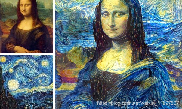
太棒了吧? 让我们看看它在PyTorch中的实现。 该过程包括六个步骤:
- 从两个输入图像中提取低级特征。 这可以使用预训练的深度学习模型来完成,例如VGG19。
from torchvision import models
# get the features portion from VGG19
vgg = models.vgg19(pretrained=True).features

# freeze all VGG parameters
for param in vgg.parameters():
    param.requires_grad_(False)
# check if GPU is available
device = torch.device("cpu")
if torch.cuda.is_available():
    device = torch.device("cuda")
vgg.to(device)
- 将两个图像加载到设备上并从VGG获取功能。 此外,应用转换:调整大小到张量,并标准化值。
from torchvision import transforms as tf
def transformation(img):
    tasks = tf.Compose([tf.Resize(400), tf.ToTensor(),
               tf.Normalize((0.44,0.44,0.44),(0.22,0.22,0.22))])
    img = tasks(img)[:3,:,:].unsqueeze(0)
    return img
img1 = Image.open("image1.jpg").convert('RGB')
img2 = Image.open("image2.jpg").convert('RGB')
img1 = transformation(img1).to(device)
img2 = transformation(img2).to(device)

- 现在,我们需要获得两个图像的相关功能。 从第一张图片中,我们需要提取与上下文或存在的对象相关的特征。 从第二张图片中,我们需要提取与样式和纹理相关的特征。
对象相关特性:在原始论文中,作者提出可以从网络的初始层提取有关对象和上下文的更有价值的信息。 这是因为在较高层中,信息空间变得更复杂并且丢失了详细的像素信息。
样式相关特征:为了从第二个图像获得纹理信息,作者使用了不同层中不同特征之间的相关性。 这在下面的第4点中详细解释。
但在到达那里之前,让我们来看看典型的VGG19型号的结构:
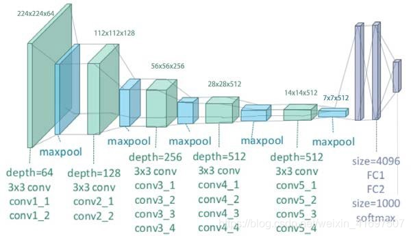
对于对象信息提取,Conv42是感兴趣的层。 它存在于深度为512的第四个卷积块中。对于样式表示,感兴趣的层是网络中每个卷积块的第一个卷积层,即conv11,conv21,conv31,conv41和conv51。 这些层是纯粹基于作者的实验选择的,我只是在本文中复制它们的结果。
def get_features(image, model):
    layers = {'0': 'conv1_1', '5': 'conv2_1',  '10': 'conv3_1',
              '19': 'conv4_1', '21': 'conv4_2', '28': 'conv5_1'}
    x = image
    features = {}
    for name, layer in model._modules.items():
        x = layer(x)
        if name in layers:
            features[layers[name]] = x
    return features
img1_features = get_features(img1, vgg)
img2_features = get_features(img2, vgg)
- 如前所述,作者使用不同层次的相关性来获得与样式相关的特征。 这些特征相关性由Gram矩阵G给出,其中G中的每个单元(i,j)是层中的矢量化特征映射i和j之间的内积。
def correlation_matrix(tensor):
    _, d, h, w = tensor.size()
    tensor = tensor.view(d, h * w)
    correlation = torch.mm(tensor, tensor.t())
    return correlation
correlations = {l: correlation_matrix(img2_features[l]) for l in
                                                    img2_features}
-我们终于可以使用这些功能和相关性来执行样式传输。 现在,为了将样式从一个图像转移到另一个图像,我们需要设置用于获取样式特征的每个图层的权重。 如上所述,初始图层提供了更多信息,因此我们将为这些图层设置更多权重。 此外,定义优化器函数和目标图像,它将是image1的副本。
weights = {'conv1_1': 1.0, 'conv2_1': 0.8, 'conv3_1': 0.25,
           'conv4_1': 0.21, 'conv5_1': 0.18}

target = img1.clone().requires_grad_(True).to(device)
optimizer = optim.Adam([target], lr=0.003)
- 启动损失最小化过程,在该过程中我们运行循环以执行大量步骤,并计算与对象特征提取和样式特征提取相关的损失。 使用最小化的损失,更新网络参数,其进一步更新目标图像。 经过一些迭代后,将生成更新的图像。
for ii in range(1, 2001):

    ## calculate the content loss (from image 1 and target)
    target_features = get_features(target, vgg)
    loss = target_features['conv4_2'] - img1_features['conv4_2']
    content_loss = torch.mean((loss)**2)

    ## calculate the style loss (from image 2 and target)
    style_loss = 0
    for layer in weights:

        target_feature = target_features[layer]
        target_corr = correlation_matrix(target_feature)
        style_corr = correlations[layer]

        layer_loss = torch.mean((target_corr - style_corr)**2)
        layer_loss *= weights[layer]

        _, d, h, w = target_feature.shape
        style_loss += layer_loss / (d * h * w)

    total_loss = 1e6 * style_loss + content_loss

    optimizer.zero_grad()
    total_loss.backward()
    optimizer.step()
最后,我们可以查看预测结果。 我只运行了少量的迭代,但是最多可以运行3000次迭代(如果计算资源没有吧!)。
def tensor_to_image(tensor):
    image = tensor.to("cpu").clone().detach()
    image = image.numpy().squeeze()
    image = image.transpose(1, 2, 0)
    image *= np.array((0.22, 0.22, 0.22))
                       + np.array((0.44, 0.44, 0.44))
    image = image.clip(0, 1)
    return image
fig, (ax1, ax2) = plt.subplots(1, 2, figsize=(20, 10))
ax1.imshow(tensor_to_image(img1))
ax2.imshow(tensor_to_image(target))

End Notes
PyTorch可以使用并且已经使用过很多其他用例。 它很快成为全球研究人员的宠儿。 您现在将看到的大多数开源库和开发都在GitHub上提供了PyTorch实现。
在本文中,我已经说明了PyTorch是什么以及如何开始在不同的用例中实现它。 人们应该将本指南视为起点。 通过更多数据,更精细的网络参数调整,最重要的是,在构建网络架构的同时应用创造性技能,可以提高每个用例的性能。 感谢阅读,并在下面的评论部分留下您的反馈。
References
Official PyTorch Guide: https://pytorch.org/tutorials/
Deep Learning with PyTorch: https://pytorch.org/tutorials/beginner/deep_learning_60min_blitz.html
Faizan’s Article on AnalyticsVidhya: https://www.analyticsvidhya.com/blog/2018/02/pytorch-tutorial/
Udacity Deeplearning using Pytorch: https://github.com/udacity/deep-learning-v2-pytorch
Image Style Transfer Original Paper: https://www.cv-foundation.org/openaccess/content_cvpr_2016/papers/Gatys_Image_Style_Transfer_CVPR_2016_paper.pdf