版权声明:本文为博主原创文章,未经博主允许不得转载。 https://blog.csdn.net/Forlogen/article/details/89463914
A
p
a
p
e
r
a
d
a
y
k
e
e
p
s
t
r
o
u
b
l
e
a
w
a
y
​
\color{lime}{A\ paper\ a\ day\ keeps\ trouble\ away\!}
A p a p e r a d a y k e e p s t r o u b l e a w a y 论文地址:https://arxiv.org/pdf/1711.05139v6.pdf
从题目中我们可以看出这是一篇属于Image-to-Image方面的文章,作者提出了一种新的GAN的变体,称为XGAN(GAN架构的形状像一个X),实现了在无监督学习的方式下,完成不同域(domain)的图像之间的转换。在GAN的诸多变体中,类似的有CycleGAN、DualGAN、DiscoGAN以及使用CGAN做Image-to-Image等等很多的方法,作者在实验部分也和CycleGAN进行了对比,显示了XGAN的改进效果。
XGAN中和CycleGAN相比而言,最大的改变就是它使用了语义一致性损失(semantic-consistency loss)从而保留了图像在语义级别的特征信息,而在CycleGAN中关注的是pixel层级的一致性损失,所以XGAN可以保留更高层次的特征信息,生成的图像的结果更加的好。
下面我们主要看一下XGAN的模型架构和损失函数,其他导引的部分,具体可见原论文。
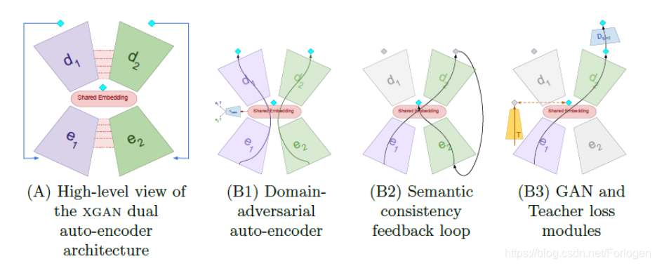
首先看一下它的架构,如下所示
从上图中我们可以大致的看出,XGAN其实就是两个Auto-encoder的组合,通过设置不同的损失项添加约束来达到Image-to-Image的效果。
其中,
D
1
、
D
2
D_{1}、D_{2}
D 1 、 D 2
e
1
、
e
2
e_{1}、e_{2}
e 1 、 e 2
d
1
、
d
2
d_{1}、d_{2}
d 1 、 d 2
s
h
a
r
e
d
E
m
b
e
d
d
i
n
g
shared\ Embedding
s h a r e d E m b e d d i n g
模型的架构看起来并不复杂,那么它是如何优于CycleGAN及其他的类似的模型的呢?XGAN优于其他模型的关键在于损失函数的设计,它包含有五个主要的损失项:
重建损失项
L
r
e
c
\mathcal{L}_{rec}
L r e c
L
r
e
c
,
1
=
E
x
∼
p
D
1
(
∥
x
−
d
1
(
e
1
(
x
)
)
∥
2
)
L
r
e
c
,
2
=
E
x
∼
p
D
2
(
∥
x
−
d
2
(
e
2
(
x
)
)
∥
2
)
L
r
e
c
=
L
r
e
c
,
1
+
L
r
e
c
,
2
\mathcal{L}_{r e c, 1}=\mathbb{E}_{\mathbf{x} \sim p_{\mathcal{D}_{1}}}\left(\left\|\mathbf{x}-d_{1}\left(e_{1}(\mathbf{x})\right)\right\|_{2}\right) \\\mathcal{L}_{r e c, 2}=\mathbb{E}_{\mathbf{x} \sim p_{\mathcal{D}_{2}}}\left(\left\|\mathbf{x}-d_{2}\left(e_{2}(\mathbf{x})\right)\right\|_{2}\right) \\\mathcal{L}_{r e c}=\mathcal{L}_{r e c, 1}+\mathcal{L}_{r e c, 2}
L r e c , 1 = E x ∼ p D 1 ( ∥ x − d 1 ( e 1 ( x ) ) ∥ 2 ) L r e c , 2 = E x ∼ p D 2 ( ∥ x − d 2 ( e 2 ( x ) ) ∥ 2 ) L r e c = L r e c , 1 + L r e c , 2
x
x
x
∣
∣
.
∣
∣
||.||
∣ ∣ . ∣ ∣
域对抗损失
L
d
a
n
n
\mathcal{L}_{dann}
L d a n n
e
1
e_{1}
e 1
e
2
e_{2}
e 2
c
d
a
n
n
c_{dann}
c d a n n
e
1
e_{1}
e 1
e
2
e_{2}
e 2
L
d
a
n
n
\mathcal{L}_{dann}
L d a n n
min
θ
e
1
,
θ
e
2
max
θ
d
a
n
n
L
d
a
n
n
,
where
L
d
a
n
n
=
E
p
D
1
ℓ
(
1
,
c
d
a
n
n
(
e
1
(
x
)
)
)
+
E
p
D
2
ℓ
(
2
,
c
d
a
n
n
(
e
2
(
x
)
)
)
\begin{array}{l}{\min _{\theta_{e_{1}}, \theta_{e_{2}}} \max _{\theta_{d a n n}} \mathcal{L}_{d a n n}, \text { where }} \\ {\mathcal{L}_{d a n n}=\mathbb{E}_{p_{\mathcal{D}_{1}}} \ell\left(1, c_{d a n n}\left(e_{1}(\mathrm{x})\right)\right)+\mathbb{E}_{p_{\mathcal{D}_{2}}} \ell\left(2, c_{d a n n}\left(e_{2}(\mathrm{x})\right)\right)}\end{array}
min θ e 1 , θ e 2 max θ d a n n L d a n n , where L d a n n = E p D 1 ℓ ( 1 , c d a n n ( e 1 ( x ) ) ) + E p D 2 ℓ ( 2 , c d a n n ( e 2 ( x ) ) )
语义一致性损失
L
s
e
m
\mathcal{L}_{sem}
L s e m
L
s
e
m
,
1
→
2
=
E
x
∼
p
D
1
∥
e
1
(
x
)
−
e
2
(
g
1
→
2
(
x
)
)
∥
,
likewise for
L
s
e
m
,
2
→
1
∥
⋅
∥
denotes a distance between vectors.
\begin{array}{l}{\mathcal{L}_{s e m, 1 \rightarrow 2}=\mathbb{E}_{\mathbf{x} \sim p_{\mathcal{D}_{1}}}\left\|e_{1}(\mathbf{x})-e_{2}\left(g_{1 \rightarrow 2}(\mathbf{x})\right)\right\|, \text { likewise for } \mathcal{L}_{s e m, 2 \rightarrow 1}} \\ {\|\cdot\| \text { denotes a distance between vectors. }}\end{array}
L s e m , 1 → 2 = E x ∼ p D 1 ∥ e 1 ( x ) − e 2 ( g 1 → 2 ( x ) ) ∥ , likewise for L s e m , 2 → 1 ∥ ⋅ ∥ denotes a distance between vectors.
生成对抗损失
L
g
a
n
\mathcal{L}_{gan}
L g a n
min
θ
g
1
→
2
max
θ
1
→
2
L
g
a
n
,
1
→
2
L
g
a
n
,
1
→
2
=
E
x
∼
p
D
(
log
(
D
1
→
2
(
x
)
)
)
+
E
x
∼
p
D
1
(
log
(
1
−
D
1
→
2
(
g
1
→
2
(
x
)
)
)
)
)
Likewise
L
g
a
n
,
2
→
1
i
s
d
e
f
i
n
e
d
f
o
r
t
h
e
t
r
a
n
s
f
o
r
m
a
t
i
o
n
f
r
o
m
D
2
t
o
D
1
.
\begin{array}{l}{\min _{\theta_{g_{1 \rightarrow 2}}} \max _{\theta_{1 \rightarrow 2}} \mathcal{L}_{g a n, 1 \rightarrow 2}} \\ {\mathcal{L}_{g a n, 1 \rightarrow 2}=\mathbb{E}_{\mathrm{x} \sim p_{\mathcal{D}}}\left(\log \left(D_{1 \rightarrow 2}(\mathrm{x})\right)\right)+\mathbb{E}_{\mathrm{x} \sim p_{\mathcal{D}_{1}}}\left(\log \left(1-D_{1 \rightarrow 2}\left(g_{1 \rightarrow 2}(\mathrm{x})\right)\right)\right) )}\end{array} \\ \text { Likewise}\ \mathcal{L}_{g a n,2\rightarrow 1}\ is defined\ for\ the\ transformation\ from\ D_{2}\ to\ D_{1}.
min θ g 1 → 2 max θ 1 → 2 L g a n , 1 → 2 L g a n , 1 → 2 = E x ∼ p D ( log ( D 1 → 2 ( x ) ) ) + E x ∼ p D 1 ( log ( 1 − D 1 → 2 ( g 1 → 2 ( x ) ) ) ) ) Likewise L g a n , 2 → 1 i s d e f i n e d f o r t h e t r a n s f o r m a t i o n f r o m D 2 t o D 1 .
指导损失
L
t
e
a
c
h
\mathcal{L}_{teach}
L t e a c h
L
teach
=
E
x
∼
p
D
1
∥
T
(
x
)
−
e
1
(
x
)
∥
where
∥
⋅
∥
is a distance between vectors.
\begin{aligned} \mathcal{L}_{\text {teach}}=& \mathbb{E}_{\mathrm{x} \sim p_{\mathcal{D}_{1}}}\left\|T(\mathrm{x})-e_{1}(\mathrm{x})\right\| \\ & \text { where }\|\cdot\| \text { is a distance between vectors. } \end{aligned}
L teach = E x ∼ p D 1 ∥ T ( x ) − e 1 ( x ) ∥ where ∥ ⋅ ∥ is a distance between vectors.
综合五个主要的损失项得到整体的损失函数为:
L
X
G
A
N
=
L
r
e
c
+
ω
d
L
d
a
n
n
+
ω
s
L
s
e
m
+
ω
g
L
g
a
n
+
ω
t
L
t
e
a
c
h
\mathcal{L}_{\mathrm{XGAN}}=\mathcal{L}_{r e c}+\omega_{d} \mathcal{L}_{d a n n}+\omega_{s} \mathcal{L}_{s e m}+\omega_{g} \mathcal{L}_{g a n}+\omega_{t} \mathcal{L}_{t e a c h}
L X G A N = L r e c + ω d L d a n n + ω s L s e m + ω g L g a n + ω t L t e a c h
ω
\omega
ω
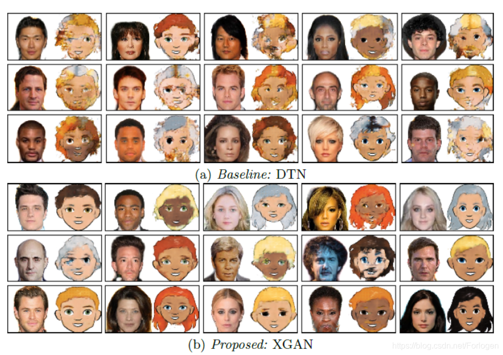
在实验部分,作者主要完成的是真实人脸和卡通人脸的转换实验,使用的两个数据集是CartoonSet(https://github.com/google/cartoonset)和VGG-Face
转换的实验结果如下所示,可以看出效果还是不错的,脸部的基本特征信息都很好的保留了下来
然后和DTN相比而言,效果要好很多。XGAN 可以更好地捕捉到图像的语义特征信息,生成的图像质量更高,虽然也有一些小问题,但总体效果要优于DTN
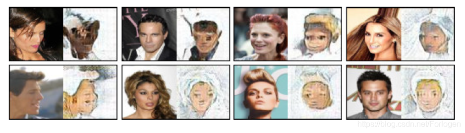
和CycleGAN的实验对比,可以看出CycleGAN生成的图像的质量要差很多
此外还通过实验证明了设置的损失项的有效性。
XGAN虽然模型的结构很简单,但是通过设置新的损失项,从一个更高的层次把握图像的特征,从而得到了更好的结果。这对于我们的研究工作具有一定的指导意义,当我们思考一个问题时,从不同的高度思考,也许就会有更好的收获。