数据集划分
sklearn数据集划分API:sklearn.model_selection.train_test_split
scikit-learn数据集API介绍
获取数据集返回的类型
# 小数据集
from sklearn.datasets import load_iris
# 获取数据
li = load_iris()

print("获取特征值:\n", li.data)
print("获取目标值:\n", li.target)
print("数据描述:\n", li.DESCR)
print("特征名:\n", li.feature_names)
print("标签名:\n", li.target_names)
获取特征值:
 [[5.1 3.5 1.4 0.2]
 [4.9 3.  1.4 0.2]
 [4.7 3.2 1.3 0.2]
 [4.6 3.1 1.5 0.2]
 [5.  3.6 1.4 0.2]
 [5.4 3.9 1.7 0.4]
 ……
 [6.7 3.  5.2 2.3]
 [6.3 2.5 5.  1.9]
 [6.5 3.  5.2 2. ]
 [6.2 3.4 5.4 2.3]
 [5.9 3.  5.1 1.8]]
获取目标值:
 [0 0 0 0 0 0 0 0 0 0 0 0 0 0 0 0 0 0 0 0 0 0 0 0 0 0 0 0 0 0 0 0 0 0 0 0 0
 0 0 0 0 0 0 0 0 0 0 0 0 0 1 1 1 1 1 1 1 1 1 1 1 1 1 1 1 1 1 1 1 1 1 1 1 1
 1 1 1 1 1 1 1 1 1 1 1 1 1 1 1 1 1 1 1 1 1 1 1 1 1 1 2 2 2 2 2 2 2 2 2 2 2
 2 2 2 2 2 2 2 2 2 2 2 2 2 2 2 2 2 2 2 2 2 2 2 2 2 2 2 2 2 2 2 2 2 2 2 2 2
 2 2]
数据描述:
 Iris Plants Database
====================

Notes
-----
Data Set Characteristics:
    :Number of Instances: 150 (50 in each of three classes)
    :Number of Attributes: 4 numeric, predictive attributes and the class
    :Attribute Information:
        - sepal length in cm
        - sepal width in cm
        - petal length in cm
        - petal width in cm
        - class:
                - Iris-Setosa
                - Iris-Versicolour
                - Iris-Virginica
    :Summary Statistics:

    ============== ==== ==== ======= ===== ====================
                    Min  Max   Mean    SD   Class Correlation
    ============== ==== ==== ======= ===== ====================
    sepal length:   4.3  7.9   5.84   0.83    0.7826
    sepal width:    2.0  4.4   3.05   0.43   -0.4194
    petal length:   1.0  6.9   3.76   1.76    0.9490  (high!)
    petal width:    0.1  2.5   1.20  0.76     0.9565  (high!)
    ============== ==== ==== ======= ===== ====================

    :Missing Attribute Values: None
    :Class Distribution: 33.3% for each of 3 classes.
    :Creator: R.A. Fisher
    :Donor: Michael Marshall (MARSHALL%[email protected])
    :Date: July, 1988

This is a copy of UCI ML iris datasets.
http://archive.ics.uci.edu/ml/datasets/Iris

The famous Iris database, first used by Sir R.A Fisher

This is perhaps the best known database to be found in the
pattern recognition literature.  Fisher's paper is a classic in the field and
is referenced frequently to this day.  (See Duda & Hart, for example.)  The
data set contains 3 classes of 50 instances each, where each class refers to a
type of iris plant.  One class is linearly separable from the other 2; the
latter are NOT linearly separable from each other.

References
----------
   - Fisher,R.A. "The use of multiple measurements in taxonomic problems"
     Annual Eugenics, 7, Part II, 179-188 (1936); also in "Contributions to
     Mathematical Statistics" (John Wiley, NY, 1950).
   - Duda,R.O., & Hart,P.E. (1973) Pattern Classification and Scene Analysis.
     (Q327.D83) John Wiley & Sons.  ISBN 0-471-22361-1.  See page 218.
   - Dasarathy, B.V. (1980) "Nosing Around the Neighborhood: A New System
     Structure and Classification Rule for Recognition in Partially Exposed
     Environments".  IEEE Transactions on Pattern Analysis and Machine
     Intelligence, Vol. PAMI-2, No. 1, 67-71.
   - Gates, G.W. (1972) "The Reduced Nearest Neighbor Rule".  IEEE Transactions
     on Information Theory, May 1972, 431-433.
   - See also: 1988 MLC Proceedings, 54-64.  Cheeseman et al"s AUTOCLASS II
     conceptual clustering system finds 3 classes in the data.
   - Many, many more ...

特征名:
 ['sepal length (cm)', 'sepal width (cm)', 'petal length (cm)', 'petal width (cm)']
标签名:
 ['setosa' 'versicolor' 'virginica']
# 大数据集
from sklearn.datasets import fetch_20newsgroups

news = fetch_20newsgroups(data_home="./news", subset="all")

print(len(news.data))
print("获取特征值:\n", news.data[0])
print("获取目标值:\n", news.target)
print("数据描述:\n", news.DESCR)
print("标签名:\n", news.target_names)
18846
获取特征值:
 From: Mamatha Devineni Ratnam <[email protected]>
Subject: Pens fans reactions
Organization: Post Office, Carnegie Mellon, Pittsburgh, PA
Lines: 12
NNTP-Posting-Host: po4.andrew.cmu.edu


I am sure some bashers of Pens fans are pretty confused about the lack
of any kind of posts about the recent Pens massacre of the Devils. Actually,
I am  bit puzzled too and a bit relieved. However, I am going to put an end
to non-PIttsburghers' relief with a bit of praise for the Pens. Man, they
are killing those Devils worse than I thought. Jagr just showed you why
he is much better than his regular season stats. He is also a lot
fo fun to watch in the playoffs. Bowman should let JAgr have a lot of
fun in the next couple of games since the Pens are going to beat the pulp out of Jersey anyway. I was very disappointed not to see the Islanders lose the final
regular season game.          PENS RULE!!!


获取目标值:
 [10  3 17 ...  3  1  7]
数据描述:
 None
标签名:
 ['alt.atheism', 'comp.graphics', 'comp.os.ms-windows.misc', 'comp.sys.ibm.pc.hardware', 'comp.sys.mac.hardware', 'comp.windows.x', 'misc.forsale', 'rec.autos', 'rec.motorcycles', 'rec.sport.baseball', 'rec.sport.hockey', 'sci.crypt', 'sci.electronics', 'sci.med', 'sci.space', 'soc.religion.christian', 'talk.politics.guns', 'talk.politics.mideast', 'talk.politics.misc', 'talk.religion.misc']
数据集进行分割
sklearn.model_selection.train_test_split(*arrays, **options)
from sklearn.model_selection import train_test_split

x_train, x_test, y_train, y_test = train_test_split(li.data, li.target, test_size=0.25)

print("训练集特征值和目标值:\n", x_train.shape, y_train.shape)
print("测试集特征值和目标值:\n", x_test.shape, y_test.shape)
训练集特征值和目标值:
 (112, 4) (112,)
测试集特征值和目标值:
 (38, 4) (38,)
KNN(K近邻算法)
定义:
如果一个样本在特征空间中的k个最相似(即特征空间中最邻近)的样本中的大多数属于某一个类别,则该样本也属于这个类别。
KNN算法既可以做回归也可以作分类,主要的区别在于最后的决策方式不同:
KNN做分类预测时,一般是选择多数表决法,即训练集里和预测的样本特征最近的K个样本,预测为里面有最多类别数的类别。
而KNN做回归时,一般是选择平均法,即最近的K个样本的样本输出的平均值作为回归预测值。
KNN的三要素:k值的选取、距离度量的方式、分类决策规则(这里仅以分类为例,回归类似)
-
k值的选取:对于K值的选取,没有固定的经验,一般是根据样本的分布选取一个较小的值,当然个人常用的方式就是当做超参数进行网格搜索
- 选择较小的k值,等价于用较小的领域中的训练实例进行预测,训练误差会减小,只有与输入实例较近或相似的训练实例才会对预测结果起作用,与此同时带来的问题是泛化误差会增大,换句话说,K值的减小就意味着整体模型变得复杂,容易发生过拟合;
- 选择较大的k值,等价于用较大领域中的训练实例进行预测,其优点是可以减少泛化误差,但缺点是训练误差会增大。这时候,与输入实例较远(不相似的)训练实例也会对预测器作用,使预测发生错误,且K值的增大就意味着整体的模型变得简单。
-
距离度量方式:一般常用的就是欧式距离啦,计算公式如下:D(x,y)=√(x1−y1)2+(x2−y2)2+…+(xn−yn)^2
-
分类决策规则:一般都是使用前面提到的多数表决法
sklearn k-近邻算法API
-
sklearn.neighbors.KNeighborsClassifier(n_neighbors=5,algorithm=‘auto’)
- n_neighbors:int,可选(默认= 5),k_neighbors查询默认使用的邻居数
- algorithm:{‘auto’,‘ball_tree’,‘kd_tree’,‘brute’},可选用于计算最近邻居的算法:‘ball_tree’将会使用 BallTree,‘kd_tree’将使用 KDTree。‘auto’将尝试根据传递给fit方法的值来决定最合适的算法。 (不同实现方式影响效率)
from sklearn.datasets import load_iris
from sklearn.preprocessing import StandardScaler
from sklearn.model_selection import train_test_split
from sklearn.neighbors import KNeighborsClassifier
from matplotlib import pyplot as plt
# 导入数据
ir = load_iris()
X = ir.data
y = ir.target
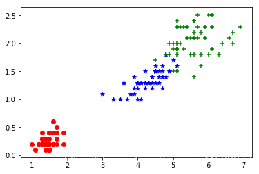
# 绘制数据分布图
# 1、X的第1、2个特征
fig = plt.figure()
plt.scatter(X[y==0, 0],X[y==0, 1],color = 'r',marker='o')
plt.scatter(X[y==1, 0],X[y==1, 1],color = 'b',marker='*')
plt.scatter(X[y==2, 0],X[y==2, 1],color = 'g',marker='+')
plt.show()
# X的第3、4个特征
plt.scatter(X[y==0, 2],X[y==0, 3],color = 'r',marker='o')
plt.scatter(X[y==1, 2],X[y==1, 3],color = 'b',marker='*')
plt.scatter(X[y==2, 2],X[y==2, 3],color = 'g',marker='+')
plt.show()

# 数据预处理:标准化
from sklearn.preprocessing import StandardScaler

std = StandardScaler()
X = std.fit_transform(X)

print("标准化后的结果:\n", X)
print("均值:\n", std.mean_)
print("标准差:\n", std.scale_)
标准化后的结果:
 [[-9.00681170e-01  1.03205722e+00 -1.34127240e+00 -1.31297673e+00]
 [-1.14301691e+00 -1.24957601e-01 -1.34127240e+00 -1.31297673e+00]
 [-1.38535265e+00  3.37848329e-01 -1.39813811e+00 -1.31297673e+00]
 [-1.50652052e+00  1.06445364e-01 -1.28440670e+00 -1.31297673e+00]
 [-1.02184904e+00  1.26346019e+00 -1.34127240e+00 -1.31297673e+00]
								 ……
 [ 7.95669016e-01 -1.24957601e-01  8.19624347e-01  1.05353673e+00]
 [ 4.32165405e-01  8.00654259e-01  9.33355755e-01  1.44795564e+00]
 [ 6.86617933e-02 -1.24957601e-01  7.62758643e-01  7.90590793e-01]]
均值:
 [5.84333333 3.054      3.75866667 1.19866667]
标准差:
 [0.82530129 0.43214658 1.75852918 0.76061262]
# 查看一下每个特征维度的方差比例
from sklearn.decomposition import PCA

pca = PCA(n_components=4)

pca.fit_transform(X)

print("每个特征维度的方差比例:\n", pca.explained_variance_ratio_)
print("每个特征维度的方差:\n", pca.explained_variance_)
每个特征维度的方差比例:
 [0.72770452 0.23030523 0.03683832 0.00515193]
每个特征维度的方差:
 [2.93035378 0.92740362 0.14834223 0.02074601]
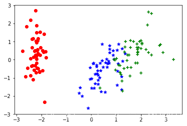
# 对数据进行降维处理,保留95%的数据量
from sklearn.decomposition import PCA
from matplotlib import pyplot as plt

pca = PCA(n_components=0.95)

_X = pca.fit_transform(X)

print("每个特征维度的方差比例:\n", pca.explained_variance_ratio_)
print("每个特征维度的方差:\n", pca.explained_variance_)
print("降维后的特征数:\n", pca.n_components_)

fig = plt.figure()
plt.scatter(_X[y==0, 0], _X[y==0, 1], color = 'r', marker='o')
plt.scatter(_X[y==1, 0], _X[y==1, 1], color = 'b', marker='*')
plt.scatter(_X[y==2, 0], _X[y==2, 1], color = 'g', marker='+')
plt.show()
每个特征维度的方差比例:
 [0.72770452 0.23030523]
每个特征维度的方差:
 [2.93035378 0.92740362]
降维后的特征数:
 2
# 分割数据集
from sklearn.model_selection import train_test_split

x_train, x_test, y_train, y_test = train_test_split(_X, y, test_size=0.25)

print(x_train.shape)
print(x_test.shape)
(112, 2)
(38, 2)
# KNN
from sklearn.neighbors import KNeighborsClassifier

knn = KNeighborsClassifier()
knn.fit(x_train, y_train)
y_pre = knn.predict(x_test)

print("测试集:\n", y_test)
print("预测:\n", y_pre)
print(knn.score(x_test, y_test))
测试集:
 [2 1 0 2 0 0 1 2 1 2 1 0 2 2 0 1 2 1 2 0 2 2 2 0 2 0 2 1 0 1 2 2 1 0 0 1 1
 0]
预测:
 [2 1 0 2 0 0 1 1 1 2 1 0 2 2 0 1 2 1 2 0 2 2 2 0 2 0 2 1 0 1 1 1 1 0 0 1 1
 0]
0.9210526315789473
# 使用网格搜索进行参数优化
from sklearn.neighbors import KNeighborsClassifier
from sklearn.model_selection import GridSearchCV

knn = KNeighborsClassifier()

params = {"n_neighbors": list(range(1,20))}
gc = GridSearchCV(knn, param_grid=params, cv=10)  # 十字交叉验证
gc.fit(x_train, y_train)

print("在测试集上准确率:\n", gc.score(x_test, y_test))
print("在交叉验证当中最好的结果:\n", gc.best_score_)
print("选择最好的模型是:\n", gc.best_estimator_)
print("每个超参数每次交叉验证的结果:\n", gc.cv_results_)
在测试集上准确率:
 0.9210526315789473
在交叉验证当中最好的结果:
 0.9375
选择最好的模型是:
 KNeighborsClassifier(algorithm='auto', leaf_size=30, metric='minkowski',
           metric_params=None, n_jobs=1, n_neighbors=10, p=2,
           weights='uniform')
每个超参数每次交叉验证的结果:
 {'split4_test_score': array([0.83333333, 0.83333333, 0.83333333, 0.75      , 0.83333333,
       0.83333333, 0.83333333, 0.83333333, 0.83333333, 0.83333333,
       0.83333333, 0.83333333, 0.83333333, 0.83333333, 0.83333333,
       0.75      , 0.75      , 0.75      , 0.75      ]), 'split2_test_score': array([0.91666667, 0.91666667, 0.91666667, 0.91666667, 0.91666667,
       0.91666667, 0.91666667, 0.91666667, 0.91666667, 0.91666667,
       0.91666667, 0.91666667, 0.91666667, 0.91666667, 0.91666667,
       0.91666667, 0.91666667, 0.91666667, 0.91666667]), 'split9_train_score': array([1.        , 0.93203883, 0.94174757, 0.91262136, 0.93203883,
       0.91262136, 0.91262136, 0.93203883, 0.9223301 , 0.9223301 ,
       0.9223301 , 0.93203883, 0.9223301 , 0.93203883, 0.91262136,
       0.93203883, 0.93203883, 0.9223301 , 0.91262136]), 'mean_fit_time': array([0.00050001, 0.0002975 , 0.        , 0.00050042, 0.00040083,
       0.        , 0.        , 0.00085793, 0.        , 0.        ,
       0.        , 0.00120976, 0.00045214, 0.00050051, 0.        ,
       0.        , 0.        , 0.        , 0.00060329]), 'std_test_score': array([0.10104714, 0.09836994, 0.07909462, 0.08683969, 0.06165686,
       0.05317918, 0.0724194 , 0.06165686, 0.06453475, 0.05408752,
       0.07100456, 0.06453475, 0.07100456, 0.07954131, 0.06294293,
       0.09200407, 0.09237094, 0.08821965, 0.08821965]), 'split7_test_score': array([0.81818182, 0.72727273, 0.72727273, 0.72727273, 0.81818182,
       0.90909091, 0.81818182, 0.81818182, 0.81818182, 0.90909091,
       0.81818182, 0.81818182, 0.81818182, 0.90909091, 0.90909091,
       0.90909091, 0.90909091, 0.90909091, 0.90909091]), 'split0_train_score': array([1.  , 0.93, 0.94, 0.91, 0.91, 0.91, 0.92, 0.92, 0.91, 0.93, 0.92,
       0.92, 0.91, 0.91, 0.92, 0.91, 0.92, 0.91, 0.9 ]), 'mean_score_time': array([0.00129406, 0.00049615, 0.00030077, 0.00070465, 0.00060208,
       0.00040076, 0.00095274, 0.        , 0.00140512, 0.        ,
       0.00080147, 0.00100615, 0.00110621, 0.00090182, 0.00030046,
       0.        , 0.00106623, 0.        , 0.        ]), 'split1_test_score': array([0.91666667, 0.91666667, 0.91666667, 0.91666667, 0.91666667,
       0.91666667, 0.91666667, 0.91666667, 0.91666667, 0.91666667,
       0.91666667, 0.91666667, 0.91666667, 0.91666667, 0.91666667,
       0.91666667, 0.91666667, 0.91666667, 0.91666667]), 'split3_train_score': array([1.  , 0.92, 0.92, 0.92, 0.93, 0.93, 0.93, 0.92, 0.93, 0.93, 0.94,
       0.93, 0.93, 0.92, 0.93, 0.93, 0.93, 0.92, 0.92]), 'params': [{'n_neighbors': 1}, {'n_neighbors': 2}, {'n_neighbors': 3}, {'n_neighbors': 4}, {'n_neighbors': 5}, {'n_neighbors': 6}, {'n_neighbors': 7}, {'n_neighbors': 8}, {'n_neighbors': 9}, {'n_neighbors': 10}, {'n_neighbors': 11}, {'n_neighbors': 12}, {'n_neighbors': 13}, {'n_neighbors': 14}, {'n_neighbors': 15}, {'n_neighbors': 16}, {'n_neighbors': 17}, {'n_neighbors': 18}, {'n_neighbors': 19}], 'std_score_time': array([0.00118461, 0.00049618, 0.00045944, 0.00142576, 0.00180624,
       0.00120227, 0.00193534, 0.        , 0.00225458, 0.        ,
       0.00160294, 0.00206339, 0.00221244, 0.0020128 , 0.00090137,
       0.        , 0.0021644 , 0.        , 0.        ]), 'param_n_neighbors': masked_array(data=[1, 2, 3, 4, 5, 6, 7, 8, 9, 10, 11, 12, 13, 14, 15, 16,
                   17, 18, 19],
             mask=[False, False, False, False, False, False, False, False,
                   False, False, False, False, False, False, False, False,
                   False, False, False],
       fill_value='?',
            dtype=object), 'split1_train_score': array([1.  , 0.93, 0.94, 0.91, 0.93, 0.91, 0.93, 0.94, 0.91, 0.92, 0.92,
       0.93, 0.93, 0.93, 0.92, 0.93, 0.93, 0.92, 0.92]), 'split9_test_score': array([0.77777778, 0.77777778, 0.88888889, 0.88888889, 0.88888889,
       0.88888889, 1.        , 0.88888889, 1.        , 1.        ,
       1.        , 1.        , 1.        , 1.        , 1.        ,
       1.        , 1.        , 0.88888889, 0.88888889]), 'split8_train_score': array([1.        , 0.91176471, 0.93137255, 0.90196078, 0.92156863,
       0.91176471, 0.92156863, 0.92156863, 0.91176471, 0.92156863,
       0.92156863, 0.93137255, 0.92156863, 0.93137255, 0.91176471,
       0.92156863, 0.92156863, 0.91176471, 0.90196078]), 'split6_train_score': array([1.        , 0.91089109, 0.93069307, 0.89108911, 0.9009901 ,
       0.9009901 , 0.92079208, 0.92079208, 0.91089109, 0.92079208,
       0.92079208, 0.9009901 , 0.9009901 , 0.89108911, 0.9009901 ,
       0.9009901 , 0.89108911, 0.9009901 , 0.91089109]), 'mean_test_score': array([0.85714286, 0.84821429, 0.88392857, 0.88392857, 0.91964286,
       0.91071429, 0.91964286, 0.91964286, 0.92857143, 0.9375    ,
       0.91964286, 0.92857143, 0.91964286, 0.91964286, 0.92857143,
       0.91071429, 0.91071429, 0.90178571, 0.90178571]), 'split8_test_score': array([1., 1., 1., 1., 1., 1., 1., 1., 1., 1., 1., 1., 1., 1., 1., 1., 1.,
       1., 1.]), 'split5_train_score': array([1.        , 0.94059406, 0.94059406, 0.93069307, 0.93069307,
       0.93069307, 0.92079208, 0.93069307, 0.93069307, 0.94059406,
       0.93069307, 0.93069307, 0.93069307, 0.95049505, 0.93069307,
       0.92079208, 0.92079208, 0.89108911, 0.91089109]), 'std_train_score': array([0.        , 0.00888981, 0.01006128, 0.01321783, 0.01107251,
       0.01408626, 0.0058268 , 0.00776117, 0.01151369, 0.00908734,
       0.01052499, 0.01207672, 0.01092932, 0.01675674, 0.01045898,
       0.00970297, 0.01302783, 0.01239761, 0.00875891]), 'split6_test_score': array([1., 1., 1., 1., 1., 1., 1., 1., 1., 1., 1., 1., 1., 1., 1., 1., 1.,
       1., 1.]), 'split7_train_score': array([1.        , 0.92079208, 0.92079208, 0.92079208, 0.93069307,
       0.93069307, 0.93069307, 0.93069307, 0.94059406, 0.93069307,
       0.94059406, 0.94059406, 0.94059406, 0.92079208, 0.92079208,
       0.92079208, 0.91089109, 0.9009901 , 0.92079208]), 'split3_test_score': array([0.83333333, 0.83333333, 0.83333333, 0.83333333, 0.91666667,
       0.91666667, 0.91666667, 0.91666667, 0.91666667, 0.91666667,
       0.83333333, 0.91666667, 0.83333333, 0.75      , 0.83333333,
       0.75      , 0.75      , 0.75      , 0.75      ]), 'split4_train_score': array([1.  , 0.92, 0.95, 0.92, 0.94, 0.95, 0.93, 0.94, 0.94, 0.95, 0.95,
       0.95, 0.93, 0.95, 0.94, 0.93, 0.94, 0.93, 0.93]), 'std_fit_time': array([0.00067014, 0.00045446, 0.        , 0.00150125, 0.00120249,
       0.        , 0.        , 0.00189062, 0.        , 0.        ,
       0.        , 0.00241954, 0.00135641, 0.00150154, 0.        ,
       0.        , 0.        , 0.        , 0.00180988]), 'mean_train_score': array([1.        , 0.92360808, 0.93651993, 0.91571564, 0.92459837,
       0.92167623, 0.92364672, 0.92757857, 0.9226273 , 0.92959779,
       0.92859779, 0.92956886, 0.9246176 , 0.92657876, 0.92068613,
       0.92261817, 0.92263797, 0.91371641, 0.91471564]), 'split5_test_score': array([0.63636364, 0.72727273, 0.81818182, 0.90909091, 0.90909091,
       0.90909091, 0.81818182, 0.90909091, 0.90909091, 0.90909091,
       0.90909091, 0.90909091, 0.90909091, 0.90909091, 0.90909091,
       1.        , 0.90909091, 1.        , 1.        ]), 'split2_train_score': array([1.  , 0.92, 0.95, 0.94, 0.92, 0.93, 0.92, 0.92, 0.92, 0.93, 0.92,
       0.93, 0.93, 0.93, 0.92, 0.93, 0.93, 0.93, 0.92]), 'rank_test_score': array([18, 19, 16, 16,  5, 11,  5,  5,  2,  1,  5,  2,  5,  5,  2, 11, 11,
       14, 14]), 'split0_test_score': array([0.83333333, 0.75      , 0.91666667, 0.91666667, 1.        ,
       0.83333333, 1.        , 1.        , 1.        , 1.        ,
       1.        , 1.        , 1.        , 1.        , 1.        ,
       0.91666667, 1.        , 0.91666667, 0.91666667])}
# 不进行PCA降维的结果怎么样呢
from sklearn.datasets import load_iris
from sklearn.preprocessing import StandardScaler
from sklearn.model_selection import train_test_split, GridSearchCV
from sklearn.neighbors import KNeighborsClassifier

ir = load_iris()
X = ir.data
y = ir.target

std = StandardScaler()
X = std.fit_transform(X)

x_train, x_test, y_train, y_test = train_test_split(X, y, test_size=0.25)

knn = KNeighborsClassifier()

params = {"n_neighbors": list(range(1,20))}
gc = GridSearchCV(knn, param_grid=params, cv=10)

gc.fit(x_train, y_train)

print("在测试集上准确率:\n", gc.score(x_test, y_test))
print("在交叉验证当中最好的结果:\n", gc.best_score_)
print("选择最好的模型是:\n", gc.best_estimator_)
print("每个超参数每次交叉验证的结果:\n", gc.cv_results_)
在测试集上准确率:
 0.8947368421052632
在交叉验证当中最好的结果:
 0.9732142857142857
选择最好的模型是:
 KNeighborsClassifier(algorithm='auto', leaf_size=30, metric='minkowski',
           metric_params=None, n_jobs=1, n_neighbors=6, p=2,
           weights='uniform')
每个超参数每次交叉验证的结果:
 {'split4_test_score': array([0.90909091, 0.90909091, 0.90909091, 0.90909091, 0.90909091,
       0.90909091, 0.90909091, 0.90909091, 0.90909091, 0.90909091,
       0.90909091, 0.90909091, 0.90909091, 0.90909091, 0.90909091,
       0.90909091, 0.90909091, 0.90909091, 0.90909091]), 'split2_test_score': array([1., 1., 1., 1., 1., 1., 1., 1., 1., 1., 1., 1., 1., 1., 1., 1., 1.,
       1., 1.]), 'split9_train_score': array([1.        , 0.98039216, 0.97058824, 0.96078431, 0.98039216,
       0.97058824, 0.97058824, 0.97058824, 0.97058824, 0.98039216,
       0.99019608, 0.99019608, 0.98039216, 0.98039216, 0.98039216,
       0.97058824, 0.98039216, 0.98039216, 0.98039216]), 'mean_fit_time': array([7.97247887e-04, 2.99191475e-04, 5.00345230e-04, 9.97066498e-05,
       1.30457878e-03, 2.63810158e-04, 6.03580475e-04, 0.00000000e+00,
       5.00726700e-04, 1.70741081e-03, 0.00000000e+00, 1.00386143e-03,
       0.00000000e+00, 6.05988503e-04, 7.01737404e-04, 1.00338459e-03,
       4.50277328e-04, 6.00862503e-04, 6.01053238e-04]), 'std_test_score': array([0.04296938, 0.05808492, 0.05862088, 0.06050679, 0.06062828,
       0.0578011 , 0.06062828, 0.05890454, 0.05890454, 0.03990884,
       0.03990884, 0.04296938, 0.04496388, 0.04390372, 0.04390372,
       0.05661516, 0.05635857, 0.0571883 , 0.04390372]), 'split7_test_score': array([1. , 1. , 0.9, 0.9, 1. , 1. , 1. , 1. , 1. , 1. , 1. , 1. , 1. ,
       0.9, 1. , 1. , 1. , 1. , 1. ]), 'split0_train_score': array([1.        , 0.97979798, 0.96969697, 0.95959596, 0.96969697,
       0.96969697, 0.96969697, 0.97979798, 0.97979798, 0.97979798,
       0.97979798, 0.97979798, 0.97979798, 0.95959596, 0.96969697,
       0.96969697, 0.95959596, 0.96969697, 0.96969697]), 'mean_score_time': array([0.00029898, 0.00059791, 0.00104046, 0.00039878, 0.00050261,
       0.00060213, 0.        , 0.00100594, 0.00030053, 0.00040081,
       0.00055296, 0.0004009 , 0.        , 0.        , 0.00040069,
       0.00040069, 0.00040073, 0.00040326, 0.00085547]), 'split1_test_score': array([0.92307692, 0.92307692, 0.92307692, 0.92307692, 1.        ,
       1.        , 1.        , 0.92307692, 0.92307692, 0.92307692,
       0.92307692, 0.92307692, 0.92307692, 0.92307692, 0.92307692,
       0.84615385, 0.84615385, 0.84615385, 0.92307692]), 'split3_train_score': array([1.        , 0.99009901, 0.99009901, 0.98019802, 0.98019802,
       0.99009901, 0.98019802, 0.99009901, 0.99009901, 0.98019802,
       0.97029703, 0.97029703, 0.97029703, 0.95049505, 0.95049505,
       0.95049505, 0.95049505, 0.93069307, 0.94059406]), 'params': [{'n_neighbors': 1}, {'n_neighbors': 2}, {'n_neighbors': 3}, {'n_neighbors': 4}, {'n_neighbors': 5}, {'n_neighbors': 6}, {'n_neighbors': 7}, {'n_neighbors': 8}, {'n_neighbors': 9}, {'n_neighbors': 10}, {'n_neighbors': 11}, {'n_neighbors': 12}, {'n_neighbors': 13}, {'n_neighbors': 14}, {'n_neighbors': 15}, {'n_neighbors': 16}, {'n_neighbors': 17}, {'n_neighbors': 18}, {'n_neighbors': 19}], 'std_score_time': array([0.00045669, 0.00048819, 0.00070925, 0.0004884 , 0.00120886,
       0.00180638, 0.        , 0.00206248, 0.00090158, 0.00120242,
       0.00165889, 0.0012027 , 0.        , 0.        , 0.00120206,
       0.00120206, 0.0012022 , 0.00120115, 0.00188583]), 'param_n_neighbors': masked_array(data=[1, 2, 3, 4, 5, 6, 7, 8, 9, 10, 11, 12, 13, 14, 15, 16,
                   17, 18, 19],
             mask=[False, False, False, False, False, False, False, False,
                   False, False, False, False, False, False, False, False,
                   False, False, False],
       fill_value='?',
            dtype=object), 'split1_train_score': array([1.        , 0.98989899, 0.95959596, 0.97979798, 0.95959596,
       0.97979798, 0.98989899, 0.98989899, 0.97979798, 0.96969697,
       0.98989899, 0.96969697, 0.97979798, 0.96969697, 0.97979798,
       0.95959596, 0.96969697, 0.94949495, 0.94949495]), 'split9_test_score': array([1. , 1. , 0.9, 0.9, 0.9, 1. , 0.9, 1. , 1. , 1. , 1. , 1. , 0.9,
       1. , 0.9, 0.9, 0.9, 0.9, 0.9]), 'split8_train_score': array([1.        , 0.98039216, 0.97058824, 0.96078431, 0.97058824,
       0.97058824, 0.97058824, 0.97058824, 0.97058824, 0.98039216,
       0.99019608, 0.99019608, 0.98039216, 0.98039216, 0.97058824,
       0.95098039, 0.95098039, 0.96078431, 0.97058824]), 'split6_train_score': array([1.        , 0.97029703, 0.98019802, 0.97029703, 0.97029703,
       0.98019802, 0.97029703, 0.98019802, 0.98019802, 0.99009901,
       0.99009901, 0.98019802, 0.99009901, 0.97029703, 0.98019802,
       0.96039604, 0.97029703, 0.93069307, 0.94059406]), 'mean_test_score': array([0.96428571, 0.94642857, 0.9375    , 0.94642857, 0.96428571,
       0.97321429, 0.96428571, 0.96428571, 0.96428571, 0.97321429,
       0.97321429, 0.96428571, 0.95535714, 0.96428571, 0.96428571,
       0.94642857, 0.96428571, 0.95535714, 0.96428571]), 'split8_test_score': array([1., 1., 1., 1., 1., 1., 1., 1., 1., 1., 1., 1., 1., 1., 1., 1., 1.,
       1., 1.]), 'split5_train_score': array([1.        , 0.97029703, 0.97029703, 0.96039604, 0.98019802,
       0.96039604, 0.97029703, 0.96039604, 0.96039604, 0.98019802,
       0.97029703, 0.96039604, 0.96039604, 0.95049505, 0.96039604,
       0.95049505, 0.96039604, 0.95049505, 0.95049505]), 'std_train_score': array([0.        , 0.00760821, 0.00806748, 0.00854338, 0.00782063,
       0.00911245, 0.00652623, 0.00987484, 0.00765306, 0.0064652 ,
       0.00909317, 0.01128602, 0.01065906, 0.01076006, 0.00935867,
       0.00989672, 0.009099  , 0.01855277, 0.01442204]), 'split6_test_score': array([0.90909091, 0.90909091, 0.90909091, 1.        , 1.        ,
       1.        , 1.        , 1.        , 1.        , 1.        ,
       1.        , 0.90909091, 0.90909091, 0.90909091, 0.90909091,
       0.90909091, 1.        , 1.        , 1.        ]), 'split7_train_score': array([1.        , 0.97058824, 0.98039216, 0.96078431, 0.96078431,
       0.97058824, 0.97058824, 0.97058824, 0.98039216, 0.99019608,
       0.98039216, 0.97058824, 0.97058824, 0.97058824, 0.97058824,
       0.97058824, 0.97058824, 0.97058824, 0.97058824]), 'split3_test_score': array([0.90909091, 0.81818182, 0.81818182, 0.81818182, 0.81818182,
       0.81818182, 0.81818182, 0.81818182, 0.81818182, 0.90909091,
       0.90909091, 0.90909091, 0.90909091, 1.        , 1.        ,
       0.90909091, 1.        , 0.90909091, 0.90909091]), 'split4_train_score': array([1.        , 0.99009901, 0.97029703, 0.98019802, 0.98019802,
       0.99009901, 0.98019802, 0.99009901, 0.98019802, 0.99009901,
       1.        , 1.        , 1.        , 0.98019802, 0.97029703,
       0.98019802, 0.97029703, 0.99009901, 0.98019802]), 'std_fit_time': array([0.00059656, 0.00045702, 0.00080724, 0.00029912, 0.00272593,
       0.00079143, 0.00181074, 0.        , 0.00150218, 0.00269693,
       0.        , 0.00205814, 0.        , 0.00181797, 0.00210521,
       0.00205689, 0.00135083, 0.00180259, 0.00180316]), 'mean_train_score': array([1.        , 0.98018616, 0.97417526, 0.9682836 , 0.97319487,
       0.97520517, 0.97423508, 0.97722538, 0.97720557, 0.98310694,
       0.98411744, 0.97913664, 0.97817606, 0.96821506, 0.96924497,
       0.9633034 , 0.96527389, 0.95929368, 0.96126417]), 'split5_test_score': array([1., 1., 1., 1., 1., 1., 1., 1., 1., 1., 1., 1., 1., 1., 1., 1., 1.,
       1., 1.]), 'split2_train_score': array([1.  , 0.98, 0.98, 0.97, 0.98, 0.97, 0.97, 0.97, 0.98, 0.99, 0.98,
       0.98, 0.97, 0.97, 0.96, 0.97, 0.97, 0.96, 0.96]), 'rank_test_score': array([ 4, 16, 19, 16,  4,  1,  4,  4,  4,  1,  1,  4, 14,  4,  4, 16,  4,
       14,  4]), 'split0_test_score': array([1.        , 0.92307692, 1.        , 1.        , 1.        ,
       1.        , 1.        , 1.        , 1.        , 1.        ,
       1.        , 1.        , 1.        , 1.        , 1.        ,
       1.        , 1.        , 1.        , 1.        ])}
小结:上面的KNN案例分别用到数据可视化、数据预处理、数据降维、数据集分割、算法实现、超参数调优,这基本上是一个机器学习项目的基本流程。