机器学习回归算法整理
相关:1.(Coursera maching-learning week1 and week2)
2.以编程提交作业展开论述。
3.个人笔记心得,以项目实践为指导。
参考:1,https://www.zybuluo.com/EtoDemerzel/note/928832
2,https://blog.csdn.net/weixin_38705903/article/details/82718818
1.Linear regression with one variable
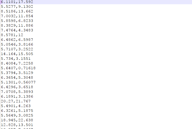
对数据说明:1,这是我们的数据集。第一列代表城市人口数据,第二列代表盈利金额。
2,数据存储在ex1data1.txt中
1.1
Ȃ>> data = load('ex1data1.txt');
>> x2 = data(:,1);
>> y2=data(:,2);
>> m=length(y2);
>> plotData(x2,y2)在命令行中执行这三句就得得到图形

1.2上面的plotData函数需要事先设计好。
function plotData(x, y)
%PLOTDATA Plots the data points x and y into a new figure
%   PLOTDATA(x,y) plots the data points and gives the figure axes labels of
%   population and profit.

figure; % open a new figure window

% ====================== YOUR CODE HERE ======================
% Instructions: Plot the training data into a figure using the
%               "figure" and "plot" commands. Set the axes labels using
%               the "xlabel" and "ylabel" commands. Assume the
%               population and revenue data have been passed in
%               as the x and y arguments of this function.
%
% Hint: You can use the 'rx' option with plot to have the markers
%       appear as red crosses. Furthermore, you can make the
%       markers larger by using plot(..., 'rx', 'MarkerSize', 10);

plot(x, y, 'rx', 'MarkerSize', 10);
xlabel('Population of City in 10,000s');
ylabel('Profit in $10,000s');

% ============================================================

end
其中核心代码也就只有几行而已
function plotData(x, y)
plot(x, y, 'rx', 'MarkerSize', 10);    //观察参数
xlabel('Population of City in 10,000s');
ylabel('Profit in $10,000s')
说明:
- 使用
plot函数绘图。用xlabel和ylabel分别设置横纵坐标的标签。rx将散点设置为红十字形(red cross) - 通过
'Markersize',10'设置散点大小
1.2
1.2 Gradient Descent
- 通过梯度下降算法计算线性回归参数 。
1.2.1 Update Equations线性回归的目标就是使代价函数最小
其中
使用批量梯度下降法(batch gradient descent ) 以使 最小。
( simultaneously update for all )
1.2.2 Implementation
目前的 是一个列向量,每一行存储一个 training example,即 。
因此在脚本文件ex1.m中,为了处理 , 给每一行增加一个 。
X = [ones(m,1) data(:,1)]; % Add a column of ones to x
因为只有一个变量 影响盈利,
初始化为
theta = zeros(2,1); % initialize fitting parameters
设置迭代次数和 的值:iterations = 1500;
alpha = 0.01;(这两个参数我现在似乎没有用上。)、
这个是调用函数的结果。
>> computeCost(x2,y2,theta)
ans =  32.073
改变参数theta的值返回的结果:
枠ɥ>> theta=[-1;2]
theta =
  -1
   2
>> computeCost(x2,y2,theta)
ans =  54.242
尝试单独调用函数:
>> gradientDescent(x2, y2, theta, alpha, iterations)
ans =
  -3.7097
   1.1743
>> theta = zeros(2,1);
>> gradientDescent(x2, y2, theta, alpha, iterations)
ans =
  -3.6303
   1.1664
结果符合。
绘制图形:
1.3 Visualizing
脚本文件ex1.m提供了对 可视化的部分。
fprintf('Visualizing J(theta_0, theta_1) ...\n')

% Grid over which we will calculate J
theta0_vals = linspace(-10, 10, 100);
theta1_vals = linspace(-1, 4, 100);
函数 linspace(BASE,LIMIT,N=100) 返回一个从BASE到LIMIT的等间距分布的行向量;如果BASE和LIMIT是列向量的话,返回一个矩阵。不输入N的时候默认为100。
% initialize J_vals to a matrix of 0 s
J_vals = zeros(length(theta0_vals), length(theta1_vals));

% Fill out J_vals
for i = 1:length(theta0_vals)
for j = 1:length(theta1_vals)
t = [theta0_vals(i); theta1_vals(j)];
J_vals(i,j) = computeCost(X, y, t);
end
end
对 和 平面上的点求出其代价函数值。
绘制曲面图:
% Because of the way meshgrids work in the surf command, we need to
% transpose J_vals before calling surf, or else the axes will be flipped
J_vals = J_vals';
% Surface plot
figure;
surf(theta0_vals, theta1_vals, J_vals)
xlabel('\theta_0'); ylabel('\theta_1');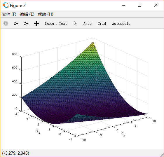
% Contour plot
figure;
% Plot J_vals as 15 contours spaced logarithmically between 0.01 and 100
contour(theta0_vals, theta1_vals, J_vals, logspace(-2, 3, 20))
xlabel('\theta_0'); ylabel('\theta_1');
hold on;
plot(theta(1), theta(2), 'rx', 'MarkerSize', 10, 'LineWidth', 2);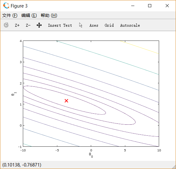
2代码天地:
单变量全过程代码:
% maching learning week2 exercise--linear regression
%-----------------Initialization---------
clear ; close all ; clc
  %clear:清除工作空间的所有变量
  %close all:关闭所有的Figure窗口
  %clc:清除命令窗口的内容,对工作环境中的全部变量无任何影响
%------------------basic Function-----------
fprintf('Running WarmUpExercise ...\n');
fprintf('5x5 Identify Matrix: \n');
warmExercise()
   %%:  function A = warmUpExercise()
   %%    A = [];
   %%    A = eye(5);
   %%  //表明这是返回一个5*5的单位矩阵。
   )
fprintf('Program paused. Press enter to continue.\n');
pause;
%-----------------Plotting----------------
fprintf('PlotData ...\n');
data = load('exadata1.txt');
X = data(:,1); %把TXT1中的第一列数据赋值到X中
y = data(:,2); %把TXT1中的第二列数据赋值到X中
m = length(y); %number of training examples
%%上面这四行是进行数据的初步处理。
plotData(X,y);
    %%//points x and y into a new figure

    %%:  function plotData(x,y)
    %%   figure;  //open a new figure window
    %%   plot(x,y,'rx','MarkerSize',10);
         %//x,y分别为轴,rx是指红色××,后面值字大小。
    %%   xlabel('Population of City in 10,000s');
    %%   ylabel('Profit in $10,000s');
    %%   end
%%-------------Cost and Gradient descent--------
X = [one(m,1),data(:,1)];
%//add a column of ones to x
theta = zeros(2,1);
%//initialize fitting parameters
iterations=1500;
alpha = 0.01;
fprintf('\nnTest the cost function...\n')
%compute and display inital cost
J = computeCost(x,y,theta);
    %%:  function J = computeCost(X,y,theta)
    %%:  m=length(y);
    %%:  J=0;
    %%   J = 1/(2*m) * sum((X*theta - y) .^ 2);
    %    //套公式
    %%   end
fprintf('With theta = [0;0]\nCost computed=%f\n',J);
fprintf('Expected cost value (approx) 32.07\n');
%further testing of the cost function
J = computeCost(X,y,[-1;2]);
fprintf('\nWith theta = [-1 ; 2]\nCost computed = %f\n', J);
fprintf('Expected cost value (approx) 54.24\n');
fprintf('Program paused. Press enter to continue.\n');
pause;
fprintf('\nRunning Gradient Descent ...\n')
%run gradient descent
theta=gradientDescent(X,y,theta,alpha,iterations);
%print theta to screen
fprintf('Theta found by gradient descent:\n');
fprintf('%f\n', theta);
fprintf('Expected theta values (approx)\n');
fprintf(' -3.6303\n  1.1664\n\n');
%Plot the liner fit
hold on;
plot(X(:,2),X*theta,'-')
%%//划直线。
legeng('Training data','Liner regression')
hold off
% don't overlay any more plots on this figure
%predict value for population sizes of 35,000 and 70,000
predict1 = [1,3.5]*theta;
fprintf('For population=35,000,we predict a profit of %f\n',...
      predict1*10000);
predict2 = [1, 7] * theta;
fprintf('For population = 70,000, we predict a profit of %f\n',...
    predict2*10000);
fprintf('Program paused. Press enter to continue.\n');
pause;
%%-----------------Visualizing J(theta_0.theta_1)----------
fprintf('Visualizing J(theta_0, theta_1) ...\n')
%calculate J
theta0_vals=linspace(-10,10,100)
%%linspace(x1,x2,n); 生成x1到x2的n个间隔相等的数,
%%如果不输入n就是默认的100个数。 就是首项x1,末项x2的等差数列
theta1_vals=linspace(-1,4,100);
%initialize J_vals to a matrix of 0's
J_val=zeros(length(theta0_vals),length(theta1_vals));
%fill out J_vals
for i =1:length(theta0_vals)
  for j=1:length(theta1_vals)
    t=[theta0_vals(i);theta1_vals(j)];
    J_vals(i,j)=computeCost(X,y,t);
  end
 end
 % Because of the way meshgrids work in the surf command, we need to
% transpose J_vals before calling surf, or else the axes will be flipped
J_vals=J_vals';
figure;
surf(theta0_vals,theta1_vals,J_vals)
xlabel('\theta_0');
ylabel('\theta_1');
%contour plot
figure;
% Plot J_vals as 15 contours
%spaced logarithmically between 0.01 and 100
contour(theta0_vals, theta1_vals, J_vals, logspace(-2, 3, 20))
xlabel('\theta_0'); ylabel('\theta_1');
hold on;
plot(theta(1), theta(2), 'rx', 'MarkerSize', 10, 'LineWidth', 2);
多变量
%%Machine Learning Online Class
%Exercise1:Liner regression with multiple variables
%week2

clear ;close all ;clc
fprintf('Loading data...\n')
data=load('ex1data2.txt');
X=data(:,1:2);  %%////后续改动地方
y=data(:,3);    %%////后续改动地方
m=length(y);
%输出自变量和因变量中的部分数据。
fprintf('First 10 examples from the dataset:\n');
fprintf('x=[%.0f %.0f],y=%.0f\n',[X(1:10,:) y(1:10,:)]');
fprintf('Program Paused. Press enter to continue.\n');
pause;     %%/////观察过程,按enter即可以继续。
%Scale feature and set them to zero mean
fprintf('Normalizing Features ....\n');
[X mu  sigma]=featureNormalize(x);  %%//标准化。
     %%:  function [X_norm,mu,sigma]=featureNormalize(X)
     %%:  X_norm=X;
     %%:  mu=zeros(1,size(X,2));
     %%         //size(X,1)->返回行数;
     %%         //size(X,2)->返回列数;
     %%:  sigma=zeros(1,size(X,2));
     %%:   mu = means(X);
     %%:   sigma=std(X);
     %%:   for i =1:size(X,1)
     %%:   X_norm(i,:)=(X(i,:)-mu)./sigma;
     %%:   end;
     %%:   end;
 %Add intercept term to X
 X=[ones(m,1)X];
 fprintf('Running gradient descent...\n');
 %choose some alpha value
 alpha = 0.01;
 num_iters = 400;
 %Init theta and run gradient descent
 theta = zeros(3,1);
 [theta ,J_history]=gradientDescentMulti(X,y,theta,alpha,num_iters);

 %绘制收敛图
 pause;
 figure;
 plot(1:numel(J_history),'-b','LineWidth',2);
 xlabel('Number of iterations');
 ylabel('Cost J');
 %%解释根据这个图进行合适选择,一般越大越好,太大就会产生新的问题。
%%If your learning rate is too large,
%%J(θ) can diverge and ‘blow up’,
%%resulting in values which are too large for computer

%display gradient descent's result
fprintf('Theta computed from gradient descent:\n');
fprintf('%f\n',theta);
fprintf('\n');
自己写:
%% Machine Learning Online Class
%  Exercise 1: Linear regression with multiple variables
%
%  Instructions
%  ------------
%
%  This file contains code that helps you get started on the
%  linear regression exercise.
%
%  You will need to complete the following functions in this
%  exericse:
%
%     warmUpExercise.m
%     plotData.m
%     gradientDescent.m
%     computeCost.m
%     gradientDescentMulti.m
%     computeCostMulti.m
%     featureNormalize.m
%     normalEqn.m
%
%  For this part of the exercise, you will need to change some
%  parts of the code below for various experiments (e.g., changing
%  learning rates).
%

%% Initialization

%% ================ Part 1: Feature Normalization ================

%% Clear and Close Figures
clear ; close all; clc
fprintf('Program paused. Press enter to continue.\n');
pause;
fprintf('Loading data ...\n');

%% Load Data
data = load('ex1data2.txt');
X = data(:, 1:2);
y = data(:, 3);
m = length(y);

% Print out some data points
fprintf('First 10 examples from the dataset: \n');
fprintf(' x = [%.0f %.0f], y = %.0f \n', [X(1:10,:) y(1:10,:)]');

fprintf('Program paused. Press enter to continue.\n');
pause;

% Scale features and set them to zero mean
fprintf('Normalizing Features ...\n');

[X mu sigma] = featureNormalize(X);
fprintf('First 10 examples after Normalizing: \n');  %%自己加的
fprintf(' x = [%.0f %.0f], y = %.0f \n', [X(1:10,:) y(1:10,:)]');
pause;


% Add intercept term to X
X = [ones(m, 1) X];


%% ================ Part 2: Gradient Descent ================

% ====================== YOUR CODE HERE ======================
% Instructions: We have provided you with the following starter
%               code that runs gradient descent with a particular
%               learning rate (alpha).
%
%               Your task is to first make sure that your functions -
%               computeCost and gradientDescent already work with
%               this starter code and support multiple variables.
%
%               After that, try running gradient descent with
%               different values of alpha and see which one gives
%               you the best result.
%
%               Finally, you should complete the code at the end
%               to predict the price of a 1650 sq-ft, 3 br house.
%
% Hint: By using the 'hold on' command, you can plot multiple
%       graphs on the same figure.
%
% Hint: At prediction, make sure you do the same feature normalization.
%

fprintf('Running gradient descent ...\n');

% Choose some alpha value

alpha = 0.01;
num_iters = 400;

% Init Theta and Run Gradient Descent
theta = zeros(3, 1);
[theta, J_history] = gradientDescentMulti(X, y, theta, alpha, num_iters);

% Plot the convergence graph
figure;
plot(1:numel(J_history), J_history, '-b', 'LineWidth', 2);
xlabel('Number of iterations');
ylabel('Cost J');

%%
% Choose some alpha value
alpha = 0.03;
num_iters = 400;

% Init Theta and Run Gradient Descent
theta = zeros(3, 1);
[theta, J_history] = gradientDescentMulti(X, y, theta, alpha, num_iters);

% Plot the convergence graph
hold on;
plot(1:numel(J_history), J_history, '-r', 'LineWidth', 2);
xlabel('Number of iterations');
ylabel('Cost J');
% Choose some alpha value
alpha = 0.1;
num_iters = 400;

% Init Theta and Run Gradient Descent
theta = zeros(3, 1);
[theta, J_history] = gradientDescentMulti(X, y, theta, alpha, num_iters);

% Plot the convergence graph
hold on;
plot(1:numel(J_history), J_history, '-g', 'LineWidth', 2);
xlabel('Number of iterations');
ylabel('Cost J');
%%


%%下面这些行对应alpha唯一为0.1.而上面是对比不同的alpha选择一个最好的。
%%%alpha = 0.1;
%%%num_iters = 400;

% Init Theta and Run Gradient Descent
%%%theta = zeros(3, 1);
%%%[theta, J_history] = gradientDescentMulti(X, y, theta, alpha, num_iters);

% Plot the convergence graph
%%%printf('press enter to plot convergence graph');
%%%pause;
%%%figure;
%%%plot(1:numel(J_history), J_history, '-b', 'LineWidth', 2);
%%%xlabel('Number of iterations');
%%%ylabel('Cost J');
%%解释根据这个图进行合适选择,一般越大越好,太大就会产生新的问题。
%%If your learning rate is too large,
%%J(θ) can diverge and ‘blow up’,
%%resulting in values which are too large for computer calculations.
%%
% Display gradient descent's result
fprintf('Theta computed from gradient descent: \n');
fprintf(' %f \n', theta);
fprintf('\n');

% Estimate the price of a 1650 sq-ft, 3 br house
% ====================== YOUR CODE HERE ======================
% Recall that the first column of X is all-ones. Thus, it does
% not need to be normalized.
%price = 0; % You should change this
ft = [1650,3];
ft=(ft-mu)./sigma;
price = [1 ft]*theta;
%%%上面三行是我加上去得到结果的。
% ============================================================

fprintf(['Predicted price of a 1650 sq-ft, 3 br house ' ...
         '(using gradient descent):\n $%f\n'], price);

fprintf('Program paused. Press enter to continue.\n');
pause;

%% ================ Part 3: Normal Equations ================

fprintf('Solving with normal equations...\n');

% ====================== YOUR CODE HERE ======================
% Instructions: The following code computes the closed form
%               solution for linear regression using the normal
%               equations. You should complete the code in
%               normalEqn.m
%
%               After doing so, you should complete this code
%               to predict the price of a 1650 sq-ft, 3 br house.
%

%% Load Data
data = csvread('ex1data2.txt');
X = data(:, 1:2);
y = data(:, 3);
m = length(y);

% Add intercept term to X
X = [ones(m, 1) X];

% Calculate the parameters from the normal equation
theta = normalEqn(X, y);
% Display normal equation's result
fprintf('Theta computed from the normal equations: \n');
fprintf(' %f \n', theta);
fprintf('\n');


% Estimate the price of a 1650 sq-ft, 3 br house
% ====================== YOUR CODE HERE ======================
%%%price = 0; % You should change this%%%%
price = [1,1650,3]*theta;


% ============================================================

fprintf(['Predicted price of a 1650 sq-ft, 3 br house ' ...
         '(using normal equations):\n $%f\n'], price);
百度代码:
%//baidu-----
%https://blog.csdn.net/sinat_40079596/article/details/79241225
%% Machine Learning Online Class
%? Exercise 1: Linear regression with multiple variables
%
%? Instructions
%? ------------
%?
%? This file contains code that helps you get started on the
%? linear regression exercise.?
%
%? You will need to complete the following functions in this?
%? exericse:
%
%? ? ?warmUpExercise.m
%? ? ?plotData.m
%? ? ?gradientDescent.m
%? ? ?computeCost.m
%? ? ?gradientDescentMulti.m
%? ? ?computeCostMulti.m
%? ? ?featureNormalize.m
%? ? ?normalEqn.m
%
%? For this part of the exercise, you will need to change some
%? parts of the code below for various experiments (e.g., changing
%? learning rates).
%


%% Initialization


%% ================ Part 1: Feature Normalization ================


%% Clear and Close Figures
clear ; close all; clc


fprintf('Loading data ...\n');


%% Load Data
data = load('ex1data2.txt');
X = data(:, 1:2);
y = data(:, 3);
m = length(y);


% Print out some data points
fprintf('First 10 examples from the dataset: \n');
fprintf(' x = [%.0f %.0f], y = %.0f \n', [X(1:10,:) y(1:10,:)]');


fprintf('Program paused. Press enter to continue.\n');
pause;


% Scale features and set them to zero mean
fprintf('Normalizing Features ...\n');


[X mu sigma] = featureNormalize(X);


% Add intercept term to X
X = [ones(m, 1) X];


%% ================ Part 2: Gradient Descent ================


% ====================== YOUR CODE HERE ======================
% Instructions: We have provided you with the following starter
%? ? ? ? ? ? ? ?code that runs gradient descent with a particular
%? ? ? ? ? ? ? ?learning rate (alpha).?
%
%? ? ? ? ? ? ? ?Your task is to first make sure that your functions -?
%? ? ? ? ? ? ? ?computeCost and gradientDescent already work with?
%? ? ? ? ? ? ? ?this starter code and support multiple variables.
%
%? ? ? ? ? ? ? ?After that, try running gradient descent with?
%? ? ? ? ? ? ? ?different values of alpha and see which one gives
%? ? ? ? ? ? ? ?you the best result.
%
%? ? ? ? ? ? ? ?Finally, you should complete the code at the end
%? ? ? ? ? ? ? ?to predict the price of a 1650 sq-ft, 3 br house.
%
% Hint: By using the 'hold on' command, you can plot multiple
%? ? ? ?graphs on the same figure.
%
% Hint: At prediction, make sure you do the same feature normalization.
%


fprintf('Running gradient descent ...\n');


% Choose some alpha value
alpha = 0.01;
num_iters = 400;


% Init Theta and Run Gradient Descent?
theta = zeros(3, 1);
[theta, J_history] = gradientDescentMulti(X, y, theta, alpha, num_iters);


% Plot the convergence graph
figure;
plot(1:numel(J_history), J_history, '-b', 'LineWidth', 2);
xlabel('Number of iterations');
ylabel('Cost J');


% Display gradient descent's result
fprintf('Theta computed from gradient descent: \n');
fprintf(' %f \n', theta);
fprintf('\n');


% Estimate the price of a 1650 sq-ft, 3 br house
% ====================== YOUR CODE HERE ======================
% Recall that the first column of X is all-ones. Thus, it does
% not need to be normalized.
ft = [1650,3];
ft = (ft - mu)./ sigma;
price = [1 ft] * theta; % You should change this 这个位置是最容易看掉的。。


% ============================================================
fprintf(['Predicted price of a 1650 sq-ft, 3 br house ' ...
         '(using gradient descent):\n $%f\n'], price);

%%%fprintf(['Predicted price of a 1650 sq-ft, 3 br house ' ...
%%% ? ? ?'(using gradient descent):\n $%f\n'], price);


fprintf('Program paused. Press enter to continue.\n');
pause;


%% ================ Part 3: Normal Equations ================


fprintf('Solving with normal equations...\n');


% ====================== YOUR CODE HERE ======================
% Instructions: The following code computes the closed form?
%? ? ? ? ? ? ? ?solution for linear regression using the normal
%? ? ? ? ? ? ? ?equations. You should complete the code in?
%? ? ? ? ? ? ? ?normalEqn.m
%
%? ? ? ? ? ? ? ?After doing so, you should complete this code?
%? ? ? ? ? ? ? ?to predict the price of a 1650 sq-ft, 3 br house.
%


%% Load Data
data = csvread('ex1data2.txt');
X = data(:, 1:2);
y = data(:, 3);
m = length(y);


% Add intercept term to X
X = [ones(m, 1) X];


% Calculate the parameters from the normal equation
theta = normalEqn(X, y);


% Display normal equation's result
fprintf('Theta computed from the normal equations: \n');
fprintf(' %f \n', theta);
fprintf('\n');


% Estimate the price of a 1650 sq-ft, 3 br house
% ====================== YOUR CODE HERE ======================
price = [1,1650,3]*theta; % You should change this


% ============================================================

fprintf(['Predicted price of a 1650 sq-ft, 3 br house ' ...
         '(using normal equations):\n $%f\n'], price);
%%%fprintf(['Predicted price of a 1650 sq-ft, 3 br house ' ...
%%%? ? ? ? ?'(using normal equations):\n $%f\n'], price);