对极几何
参考:https://blog.csdn.net/my88site/article/details/53967141
原理
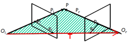
对极几何(Epipolar Geometry)描述的是两幅视图之间的内在射影关系,与外部场景无关,只依赖于摄像机内参数和这两幅试图之间的的相对姿态。假设两个相机的内部参数一致,比如焦距、镜头等,为了数学描述的方便,需引入坐标,由于坐标是人为引入的,因此客观世界中的事物可以处于不同的坐标系中。假设两个相机的X轴方向一致,像平面重叠,坐标系以左相机为准,右相机相对于左相机是简单的平移,用坐标表示为(Tx,0,0)。如下所示

实际模型
(1)本质矩阵E
推导过程


左像平面上的一点乘以本质矩阵E,结果为一条直线,该直线就是的对极线,且过在右像平面上的对应点。本质矩阵E的基本性质:秩为2,且仅依赖于外部参数R和T。其中,P表示物点矢量,p表示像点矢量。
(2)基础矩阵
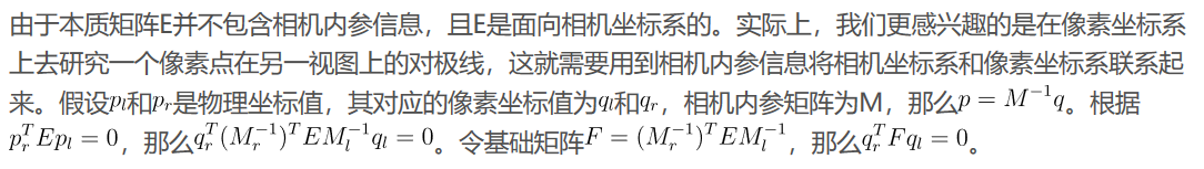
基本矩阵F求解(8点算法)
基本矩阵方程

八点法求解基本矩阵可参考 https://blog.csdn.net/a6333230/article/details/83413835
实验代码:
from PIL import Image
from numpy import *
from pylab import *
import numpy as np
from PCV.geometry import camera
from PCV.geometry import homography
from PCV.geometry import sfm
from PCV.localdescriptors import sift


# Read features
# 载入图像,并计算特征
im1 = array(Image.open('img3.jpg'))
sift.process_image('img3.jpg', 'im1.sift')
l1, d1 = sift.read_features_from_file('im1.sift')

im2 = array(Image.open('img4.jpg'))
sift.process_image('img4.jpg', 'im2.sift')
l2, d2 = sift.read_features_from_file('im2.sift')

# 匹配特征
matches = sift.match_twosided(d1, d2)
ndx = matches.nonzero()[0]

# 使用齐次坐标表示,并使用 inv(K) 归一化
x1 = homography.make_homog(l1[ndx, :2].T)
ndx2 = [int(matches[i]) for i in ndx]
x2 = homography.make_homog(l2[ndx2, :2].T)

x1n = x1.copy()
x2n = x2.copy()
print(len(ndx))

figure(figsize=(16,16))
sift.plot_matches(im1, im2, l1, l2, matches, True)
show()

# Don't use K1, and K2

#def F_from_ransac(x1, x2, model, maxiter=5000, match_threshold=1e-6):
def F_from_ransac(x1, x2, model, maxiter=5000, match_threshold=1e-6):
    """ Robust estimation of a fundamental matrix F from point
    correspondences using RANSAC (ransac.py from
    http://www.scipy.org/Cookbook/RANSAC).

    input: x1, x2 (3*n arrays) points in hom. coordinates. """

    from PCV.tools import ransac
    data = np.vstack((x1, x2))
    d = 20 # 20 is the original
    # compute F and return with inlier index
    F, ransac_data = ransac.ransac(data.T, model,
                                   8, maxiter, match_threshold, d, return_all=True)
    return F, ransac_data['inliers']

# find E through RANSAC
# 使用 RANSAC 方法估计 E
model = sfm.RansacModel()
F, inliers = F_from_ransac(x1n, x2n, model, maxiter=5000, match_threshold=1e-4)

print(len(x1n[0]))
print(len(inliers))

# 计算照相机矩阵(P2 是 4 个解的列表)
P1 = array([[1, 0, 0, 0], [0, 1, 0, 0], [0, 0, 1, 0]])
P2 = sfm.compute_P_from_fundamental(F)

# triangulate inliers and remove points not in front of both cameras
X = sfm.triangulate(x1n[:, inliers], x2n[:, inliers], P1, P2)

# plot the projection of X
cam1 = camera.Camera(P1)
cam2 = camera.Camera(P2)
x1p = cam1.project(X)
x2p = cam2.project(X)

figure()
imshow(im1)
gray()
plot(x1p[0], x1p[1], 'o')
#plot(x1[0], x1[1], 'r.')
axis('off')

figure()
imshow(im2)
gray()
plot(x2p[0], x2p[1], 'o')
#plot(x2[0], x2[1], 'r.')
axis('off')
show()

figure(figsize=(16, 16))
im3 = sift.appendimages(im1, im2)
im3 = vstack((im3, im3))

imshow(im3)

cols1 = im1.shape[1]
rows1 = im1.shape[0]
for i in range(len(x1p[0])):
    if (0<= x1p[0][i]<cols1) and (0<= x2p[0][i]<cols1) and (0<=x1p[1][i]<rows1) and (0<=x2p[1][i]<rows1):
        plot([x1p[0][i], x2p[0][i]+cols1],[x1p[1][i], x2p[1][i]],'c')
axis('off')
show()

print(F)


x1e = []
x2e = []
ers = []
for i,m in enumerate(matches):
    if m>0: #plot([locs1[i][0],locs2[m][0]+cols1],[locs1[i][1],locs2[m][1]],'c')
        x1=int(l1[i][0])
        y1=int(l1[i][1])
        x2=int(l2[int(m)][0])
        y2=int(l2[int(m)][1])
        # p1 = array([l1[i][0], l1[i][1], 1])
        # p2 = array([l2[m][0], l2[m][1], 1])
        p1 = array([x1, y1, 1])
        p2 = array([x2, y2, 1])
        # Use Sampson distance as error
        Fx1 = dot(F, p1)
        Fx2 = dot(F, p2)
        denom = Fx1[0]**2 + Fx1[1]**2 + Fx2[0]**2 + Fx2[1]**2
        e = (dot(p1.T, dot(F, p2)))**2 / denom
        x1e.append([p1[0], p1[1]])
        x2e.append([p2[0], p2[1]])
        ers.append(e)
x1e = array(x1e)
x2e = array(x2e)
ers = array(ers)

indices = np.argsort(ers)
x1s = x1e[indices]
x2s = x2e[indices]
ers = ers[indices]
x1s = x1s[:20]
x2s = x2s[:20]

figure(figsize=(16, 16))
im3 = sift.appendimages(im1, im2)
im3 = vstack((im3, im3))

imshow(im3)

cols1 = im1.shape[1]
rows1 = im1.shape[0]
for i in range(len(x1s)):
    if (0<= x1s[i][0]<cols1) and (0<= x2s[i][0]<cols1) and (0<=x1s[i][1]<rows1) and (0<=x2s[i][1]<rows1):
        plot([x1s[i][0], x2s[i][0]+cols1],[x1s[i][1], x2s[i][1]],'c')
axis('off')
show()
运行结果:
1.室外案例
sift匹配

蓝色为投影特征点,红色为原始特征点


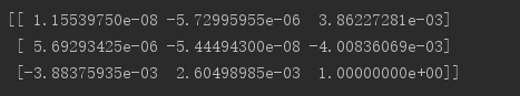
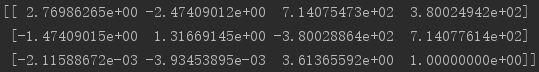
基础矩阵:
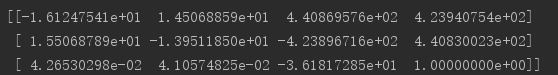
投影矩阵:
2.室内案例
sift匹配:


基础矩阵:
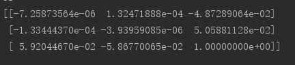
投影矩阵·: