import time
import numpy as np
import h5py
import matplotlib.pyplot as plt
import scipy
from PIL import Image
from scipy import ndimage

%matplotlib inline
plt.rcParams['figure.figsize'] = (5.0, 4.0) 
plt.rcParams['image.interpolation'] = 'nearest'
plt.rcParams['image.cmap'] = 'gray'

%load_ext autoreload
%autoreload 2

np.random.seed(1)

#引入数据（还是我们之前猫分类的数据）
train_dataset = h5py.File('datasets/train_catvnoncat.h5', "r")
train_set_x_orig = np.array(train_dataset["train_set_x"][:]) 
train_set_y_orig = np.array(train_dataset["train_set_y"][:]) 
test_dataset = h5py.File('datasets/test_catvnoncat.h5', "r")
test_set_x_orig = np.array(test_dataset["test_set_x"][:]) 
test_set_y_orig = np.array(test_dataset["test_set_y"][:])

classes = np.array(test_dataset["list_classes"][:]) 

train_set_y = train_set_y_orig.reshape((1, train_set_y_orig.shape[0]))
test_set_y = test_set_y_orig.reshape((1, test_set_y_orig.shape[0]))

#看一下数据结构
print('train_set_x_orig.shape',train_set_x_orig.shape)
print('test_set_x_orig.shape',test_set_x_orig.shape)
print('train_set_y.shape',train_set_y.shape)
print('test_set_y.shape',test_set_y.shape)

依然如此图所示把图片特征处理成1维矩阵

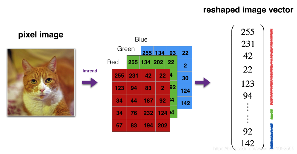
train_x_flatten = train_set_x_orig.reshape(train_set_x_orig.shape[0], -1).T   
test_x_flatten = test_set_x_orig.reshape(test_set_x_orig.shape[0], -1).T

# 标准化
train_x = train_x_flatten/255.
test_x = test_x_flatten/255.
print ("train_x's shape: " + str(train_x.shape))
print ("test_x's shape: " + str(test_x.shape))

train_x’s shape: (12288, 209)
test_x’s shape: (12288, 50)

#把所有1-4中能用到的方法都写到这里
def sigmoid(Z):    
    A = 1/(1+np.exp(-Z))
    cache = Z   
    return A, cache

def relu(Z):   
    A = np.maximum(0,Z)   
    assert(A.shape == Z.shape)   
    cache = Z 
    return A, cache

def relu_backward(dA, cache):   
    Z = cache
    dZ = np.array(dA, copy=True) 
    dZ[Z <= 0] = 0   
    assert (dZ.shape == Z.shape)   
    return dZ

def sigmoid_backward(dA, cache):
    Z = cache
    s = 1/(1+np.exp(-Z))
    dZ = dA * s * (1-s)
    assert (dZ.shape == Z.shape)
    return dZ


def initialize_parameters(n_x, n_h, n_y):
    np.random.seed(1)
    W1 = np.random.randn(n_h, n_x)*0.01
    b1 = np.zeros((n_h, 1))
    W2 = np.random.randn(n_y, n_h)*0.01
    b2 = np.zeros((n_y, 1))
    
    assert(W1.shape == (n_h, n_x))
    assert(b1.shape == (n_h, 1))
    assert(W2.shape == (n_y, n_h))
    assert(b2.shape == (n_y, 1))   
    parameters = {"W1": W1,
                  "b1": b1,
                  "W2": W2,
                  "b2": b2}   
    return parameters     


def linear_forward(A, W, b):
    
    Z = W.dot(A) + b
    assert(Z.shape == (W.shape[0], A.shape[1]))
    cache = (A, W, b)
    return Z, cache

def linear_activation_forward(A_prev, W, b, activation):
    
    
    if activation == "sigmoid":
        Z, linear_cache = linear_forward(A_prev, W, b)
        A, activation_cache = sigmoid(Z)
    
    elif activation == "relu":
        Z, linear_cache = linear_forward(A_prev, W, b)
        A, activation_cache = relu(Z)
    
    assert (A.shape == (W.shape[0], A_prev.shape[1]))
    cache = (linear_cache, activation_cache)
    return A, cache

def L_model_forward(X, parameters):
    
    caches = []
    A = X
    L = len(parameters) // 2                  
    
    for l in range(1, L):
        A_prev = A 
        A, cache = linear_activation_forward(A_prev, parameters['W' + str(l)], parameters['b' + str(l)], activation = "relu")
        caches.append(cache)
    
    AL, cache = linear_activation_forward(A, parameters['W' + str(L)], parameters['b' + str(L)], activation = "sigmoid")
    caches.append(cache)
    
    assert(AL.shape == (1,X.shape[1]))
            
    return AL, caches

def compute_cost(AL, Y):
    m = Y.shape[1]
    cost = (1./m) * (-np.dot(Y,np.log(AL).T) - np.dot(1-Y, np.log(1-AL).T))
    
    cost = np.squeeze(cost) 
    assert(cost.shape == ())
    
    return cost

def linear_backward(dZ, cache):
    
    A_prev, W, b = cache
    m = A_prev.shape[1]

    dW = 1./m * np.dot(dZ,A_prev.T)
    db = 1./m * np.sum(dZ, axis = 1, keepdims = True)
    dA_prev = np.dot(W.T,dZ)
    
    assert (dA_prev.shape == A_prev.shape)
    assert (dW.shape == W.shape)
    assert (db.shape == b.shape)
    
    return dA_prev, dW, db

def linear_activation_backward(dA, cache, activation):
    
    linear_cache, activation_cache = cache
    
    if activation == "relu":
        dZ = relu_backward(dA, activation_cache)
        dA_prev, dW, db = linear_backward(dZ, linear_cache)
        
    elif activation == "sigmoid":
        dZ = sigmoid_backward(dA, activation_cache)
        dA_prev, dW, db = linear_backward(dZ, linear_cache)
    
    return dA_prev, dW, db

def L_model_backward(AL, Y, caches):
    
    grads = {}
    L = len(caches) 
    m = AL.shape[1]
    Y = Y.reshape(AL.shape) 
    
    dAL = - (np.divide(Y, AL) - np.divide(1 - Y, 1 - AL))
    
    current_cache = caches[L-1]
    grads["dA" + str(L)], grads["dW" + str(L)], grads["db" + str(L)] = linear_activation_backward(dAL, current_cache, activation = "sigmoid")
    
    for l in reversed(range(L-1)):
        current_cache = caches[l]
        dA_prev_temp, dW_temp, db_temp = linear_activation_backward(grads["dA" + str(l + 2)], current_cache, activation = "relu")
        grads["dA" + str(l + 1)] = dA_prev_temp
        grads["dW" + str(l + 1)] = dW_temp
        grads["db" + str(l + 1)] = db_temp

    return grads

def update_parameters(parameters, grads, learning_rate):
    
    L = len(parameters) // 2 

    for l in range(L):
        parameters["W" + str(l+1)] = parameters["W" + str(l+1)] - learning_rate * grads["dW" + str(l+1)]
        parameters["b" + str(l+1)] = parameters["b" + str(l+1)] - learning_rate * grads["db" + str(l+1)]
        
    return parameters

def predict(X, y, parameters):
    m = X.shape[1]
    n = len(parameters) // 2 
    p = np.zeros((1,m))
    probas, caches = L_model_forward(X, parameters)
    for i in range(0, probas.shape[1]):
        if probas[0,i] > 0.5:
            p[0,i] = 1
        else:
            p[0,i] = 0
    print("Accuracy: "  + str(np.sum((p == y)/m)))
        
    return p

def print_mislabeled_images(classes, X, y, p):
    
    a = p + y
    mislabeled_indices = np.asarray(np.where(a == 1))
    plt.rcParams['figure.figsize'] = (40.0, 40.0) 
    num_images = len(mislabeled_indices[0])
    for i in range(num_images):
        index = mislabeled_indices[1][i]
        
        plt.subplot(2, num_images, i + 1)
        plt.imshow(X[:,index].reshape(64,64,3), interpolation='nearest')
        plt.axis('off')
        plt.title("Prediction: " + classes[int(p[0,index])].decode("utf-8") + " \n Class: " + classes[y[0,index]].decode("utf-8"))

def two_layer_model(X, Y, layers_dims, learning_rate = 0.0075, num_iterations = 3000, print_cost=False):
    
    np.random.seed(1)
    grads = {}
    #跟踪误差
    costs = []                              
    m = X.shape[1]                          
    (n_x, n_h, n_y) = layers_dims

    #初始化参数
    parameters = initialize_parameters(n_x, n_h, n_y)
    #线性参数
    W1 = parameters["W1"]
    b1 = parameters["b1"]
    W2 = parameters["W2"]
    b2 = parameters["b2"]

    #开始循环
    for i in range(0, num_iterations):
        #线性激活第一层
        A1, cache1 = linear_activation_forward(X, W1, b1, activation="relu")
        #线性激活第二层
        A2, cache2 = linear_activation_forward(A1, W2, b2, activation="sigmoid")
        #误差
        cost = compute_cost(A2, Y)
        #反向求导 在1-4中我们已经熟悉了
        dA2 = - (np.divide(Y, A2) - np.divide(1 - Y, 1 - A2))
        #线性激活反向求导
        dA1, dW2, db2 = linear_activation_backward(dA2, cache2, activation="sigmoid")
        dA0, dW1, db1 = linear_activation_backward(dA1, cache1, activation="relu")
        
        #得到梯度
        grads['dW1'] = dW1
        grads['db1'] = db1
        grads['dW2'] = dW2
        grads['db2'] = db2

        #更新参数（梯度下降）
        parameters = update_parameters(parameters, grads, learning_rate)
        #新的线性参数
        W1 = parameters["W1"]
        b1 = parameters["b1"]
        W2 = parameters["W2"]
        b2 = parameters["b2"]

        #选择是否打印
        if print_cost and i % 100 == 0:
            print("Cost after iteration {}: {}".format(i, np.squeeze(cost)))
        if print_cost and i % 100 == 0:
            costs.append(cost)

    plt.plot(np.squeeze(costs))
    plt.ylabel('cost')
    plt.xlabel('iterations (per tens)')
    plt.title("Learning rate =" + str(learning_rate))
    plt.show()

    return parameters

n_x = 12288 
n_h = 7
n_y = 1
layers_dims = (n_x, n_h, n_y)
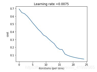
parameters = two_layer_model(train_x, train_set_y, layers_dims = (n_x, n_h, n_y), num_iterations = 2500, print_cost=True)

Cost after iteration 0: 0.693049735659989
Cost after iteration 100: 0.6464320953428849
Cost after iteration 200: 0.6325140647912678
Cost after iteration 300: 0.6015024920354665
Cost after iteration 400: 0.5601966311605747
Cost after iteration 500: 0.5158304772764729
Cost after iteration 600: 0.4754901313943325
Cost after iteration 700: 0.4339163151225749
Cost after iteration 800: 0.4007977536203886
Cost after iteration 900: 0.3580705011323798
Cost after iteration 1000: 0.3394281538366412
Cost after iteration 1100: 0.3052753636196265
Cost after iteration 1200: 0.2749137728213018
Cost after iteration 1300: 0.24681768210614868
Cost after iteration 1400: 0.19850735037466108
Cost after iteration 1500: 0.17448318112556646
Cost after iteration 1600: 0.17080762978097735
Cost after iteration 1700: 0.11306524562164687
Cost after iteration 1800: 0.09629426845937152
Cost after iteration 1900: 0.08342617959726867
Cost after iteration 2000: 0.07439078704319084
Cost after iteration 2100: 0.06630748132267933
Cost after iteration 2200: 0.05919329501038172
Cost after iteration 2300: 0.053361403485605585
Cost after iteration 2400: 0.04855478562877021

可以变换不同的学习率和迭代次数观察效果

同时也可以看一下我们的准确率

print('train',predict(train_x, train_set_y, parameters))
print('test',predict(test_x, test_set_y, parameters))

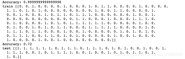
注意：您可能会注意到，在较少的迭代（例如1500）上运行模型可以提高测试集的准确性。这被称为“早期停止”，我们将在下一个课程中讨论它。提前停止是防止过度装配的一种方法。

恭喜！您的2层神经网络似乎比逻辑回归实施（70％，任务第2周）具有更好的性能（72％）。让我们看看你是否可以用L做得更好层模型。

5 - L层神经网络

使用先前的辅助函数构建，

#多层线性参数，层数由layer_dims的长度决定
def initialize_parameters_deep(layer_dims):
    #layer_dims 中的值决定了我们神经元的个数
    np.random.seed(1)
    parameters = {}
    L = len(layer_dims)          
    for l in range(1, L):
        #构建多层线性参数 需要每下一层列维度等于上一层行维度 这样满足矩阵乘法
        parameters['W' + str(l)] = np.random.randn(layer_dims[l], layer_dims[l-1]) / np.sqrt(layer_dims[l-1])
        #有多少个列维度就有多少个b
        parameters['b' + str(l)] = np.zeros((layer_dims[l], 1))
        assert(parameters['W' + str(l)].shape == (layer_dims[l], layer_dims[l-1]))
        assert(parameters['b' + str(l)].shape == (layer_dims[l], 1))     
    return parameters



layers_dims = [12288, 20, 7, 5, 1]

def L_layer_model(X, Y, layers_dims, learning_rate = 0.0075, num_iterations = 3000, print_cost=False):
    
    np.random.seed(1)
    costs = []                         
    #得到了多层的线性参数
    parameters = initialize_parameters_deep(layers_dims)
    
    for i in range(0, num_iterations):
        #多层线性+rule 最后把结果线性+sigoid
        AL, caches = L_model_forward(X, parameters)
        #计算误差
        cost = compute_cost(AL, Y)
        #反向传播
        grads = L_model_backward(AL, Y, caches)
        #梯度下降 更新参数
        parameters = update_parameters(parameters, grads, learning_rate)
        #是否输出
        if print_cost and i % 100 == 0:
            print ("Cost after iteration %i: %f" %(i, cost))
        if print_cost and i % 100 == 0:
            costs.append(cost)

    #打印成本曲线
    plt.plot(np.squeeze(costs))
    plt.ylabel('cost')
    plt.xlabel('iterations (per tens)')
    plt.title("Learning rate =" + str(learning_rate))
    plt.show()

    return parameters

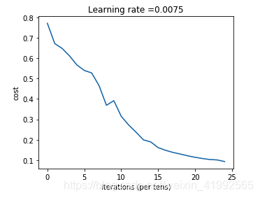
parameters = L_layer_model(train_x, train_set_y, layers_dims, num_iterations = 2500, print_cost = True)

Cost after iteration 0: 0.771749
Cost after iteration 100: 0.672053
Cost after iteration 200: 0.648263
Cost after iteration 300: 0.611507
Cost after iteration 400: 0.567047
Cost after iteration 500: 0.540138
Cost after iteration 600: 0.527930
Cost after iteration 700: 0.465477
Cost after iteration 800: 0.369126
Cost after iteration 900: 0.391747
Cost after iteration 1000: 0.315187
Cost after iteration 1100: 0.272700
Cost after iteration 1200: 0.237419
Cost after iteration 1300: 0.199601
Cost after iteration 1400: 0.189263
Cost after iteration 1500: 0.161189
Cost after iteration 1600: 0.148214
Cost after iteration 1700: 0.137775
Cost after iteration 1800: 0.129740
Cost after iteration 1900: 0.121225
Cost after iteration 2000: 0.113821
Cost after iteration 2100: 0.107839
Cost after iteration 2200: 0.102855
Cost after iteration 2300: 0.100897
Cost after iteration 2400: 0.092878

print(‘train’,predict(train_x, train_set_y, parameters))
print(‘test’,predict(test_x, test_set_y, parameters))

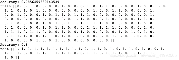
5层神经网络(80%)似乎比两层神经网络(72%)要优秀，这是因为使数据更抽象化，对于欠拟合很有效果。