文章目录
这篇博客用 python 来实线一个简单的神经网络!
参考:
- Github: https://github.com/makeyourownneuralnetwork/makeyourownneuralnetwork
- 《Python》神经网络编程——[英] Tariq Rashid 著
1 Neural Network Definition
# neural network class definition
import numpy as np
import scipy.special
class network:
    # initialise the network
    def __init__(self,input_nodes,hidden_nodes,output_nodes,learning_rate):
        self.inodes = input_nodes # the number codes of input layer
        self.hnodes = hidden_nodes # the number codes of hidden layer
        self.onodes = output_nodes # the number codes of output layer
        self.lf = learning_rate

        # initial weight 正态分布,均值0,标准差 1/sqrt(输入的节点数)
        self.whi = np.random.normal(0.0,self.inodes**(-0.5),(self.hnodes,self.inodes))  # weight between input and hidden
        self.woh = np.random.normal(0.0,self.hnodes**(-0.5),(self.onodes,self.hnodes))  # weight between input and hidden

        # activation function sigmoid
        self.activation_function = lambda x:scipy.special.expit(x)

        pass

    # train
    def train(self,input_list,target_list):
        # data
        inputs = np.array(input_list,ndmin=2).T # (x,) to (x,1)
        targets = np.array(target_list,ndmin=2).T # (x,) to (x,1)

        # forward
        hidden_inputs = np.dot(self.whi, inputs)
        hidden_outputs = self.activation_function(hidden_inputs)

        final_inputs = np.dot(self.woh, hidden_outputs)
        final_outputs = self.activation_function(final_inputs)

        # error backpropacation,/delta 的反向传播,本质就是 WT 的累乘
        output_error = targets-final_outputs
        hidden_error = np.dot(self.woh.T, output_error)

        # 更新 Woh
        self.woh += self.lf*np.dot((output_error*final_outputs*(1-final_outputs)),np.transpose(hidden_outputs))
        # 更新 Whi
        self.whi += self.lf*np.dot((hidden_error*hidden_outputs*(1-hidden_outputs)),np.transpose(inputs))

        pass

    # inference the network
    def inference(self,input_list):
        # convert inputs list to 2d array
        inputs = np.array(input_list,ndmin=2).T # (x,) to (x,1)

        hidden_inputs = np.dot(self.whi, inputs)
        hidden_outputs = self.activation_function(hidden_inputs)

        final_inputs = np.dot(self.woh, hidden_outputs)
        final_outputs = self.activation_function(final_inputs)

        return final_outputs
分为参数初始化__init__、训练 train 和推理 inference 三大部分
1)__init__ 部分
注意 weight 的初始化方式,这里采用的是
的正太分布,其中
是输入节点的个数
2)train 部分
这里是核心了,前向传播不难,难点是反向传播,具体推导可以参考 Gradient vanishing and explosion 的 demo 小节!
这里采用的是均方差损失

误差 的传播方式为 ,具体推导参考 Gradient vanishing and explosion !
3)inference 部分
同训练的时候的前向传播的过程,比较简单,可以用来测试结果!!!
2 牛刀小试
我们用 MNIST 试试,先用 train 100 test 10 的规模
2.1 Training
1)实例化网络
# create instance of neural network
input_nodes = 784
hidden_nodes = 100
output_nodes = 10
learning_rate = 0.3

n = network(input_nodes,hidden_nodes,output_nodes,learning_rate)
2)载入训练集
这个数据集是从 MNIST 抽出来的,训练 100,测试 10,
dimension,第一维是 label!!! 下载地址如下:
作者:御史神风
链接:https://www.jianshu.com/p/9842c03dc72b
来源:简书
简书著作权归作者所有,任何形式的转载都请联系作者获得授权并注明出处。
# load the traininig data
file = open("C://Users/Administrator/Desktop/mnist_train_100.csv",'r')
data_list = file.readlines()
file.close()
3)归一化图片,训练一个epoch
这里只把整个训练集训练了一次
# train
for record in data_list: #便利每一张图片
    # data
    all_values = record.split(',') # 785,第一个是 label
    scaled_input = np.asfarray(all_values[1:])/255*0.99+0.01 # normalization
    # label
    targets = np.zeros(10) + 0.01
    targets[int(all_values[0])] = 0.99
    # train
    n.train(scaled_input,targets)
2.2 Testing
1)读取数据集
# load the testing data
test_file = open("C://Users/Administrator/Desktop/mnist_test_10.csv",'r')
data_test_list = test_file.readlines()
file.close()
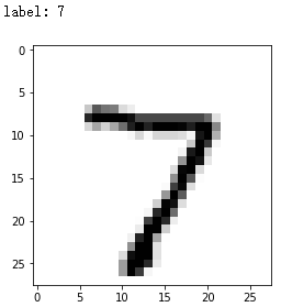
2)可以看看数据集
# test an image
import matplotlib.pylab as plt
all_test_values = data_test_list[0].split(",") # 取第一张图片
print("label:",all_test_values[0]) # label

image_array = np.asfarray(all_test_values[1:]).reshape((28,28)) # asfarra 将结构数据转化为ndarray。图片
plt.imshow(image_array,cmap='Greys',interpolation='None')
plt.show()
3)测试一张图片
n.inference(input_list=np.asfarray(all_test_values[1:])/255*0.99+0.01)
output
array([[0.17313657],
       [0.19209998],
       [0.09184129],
       [0.20961751],
       [0.23186972],
       [0.1051907 ],
       [0.08514276],
       [0.52727027],
       [0.17978829],
       [0.15776397]])
可以看到,倒数第三行对应 7 的响应最高(0-9)
4)测试所有测试集
# test images
score = []

for test_set in data_test_list:
    all_test_values = test_set.split(",")
    label = int(all_test_values[0])
    #print("label:",all_test_values[0])

    inputs = input_list=np.asfarray(all_test_values[1:])/255*0.99+0.01
    outputs = n.inference(inputs)
    predicts = np.argmax(outputs)
    #print("predict:",predicts,'\n')

    if predicts == label:
        score.append(1)
    else:
        score.append(0)

print(score)

accuracy = np.sum(score)/len(score)
accuracy
output
[1, 0, 1, 1, 1, 1, 1, 0, 0, 0]
0.6
precision 有 60%
3 Classification on whole MNIST
数据集下载地址:https://pjreddie.com/projects/mnist-in-csv/
调整下参数
# load the traininig data
file = open("C://Users/Administrator/Desktop/mnist_train.csv",'r')
data_list = file.readlines()
file.close()

# create instance of neural network
input_nodes = 784
hidden_nodes = 200
output_nodes = 10
learning_rate = 0.1

n = network(input_nodes,hidden_nodes,output_nodes,learning_rate)

# train
#for i in range(epochs):
#    print("--------------epoch%s-------------------"%i)
for record in data_list:
    # data
    all_values = record.split(',') # 785,第一个是 label
    scaled_input = np.asfarray(all_values[1:])/255*0.99+0.01
    # label
    targets = np.zeros(10) + 0.01
    targets[int(all_values[0])] = 0.99
    n.train(scaled_input,targets)

# load the testing data
test_file = open("C://Users/Administrator/Desktop/mnist_test.csv",'r')
data_test_list = test_file.readlines()
file.close()

# test images
score = []

for test_set in data_test_list:
    all_test_values = test_set.split(",")
    label = int(all_test_values[0])
    #print("label:",all_test_values[0])

    inputs = input_list=np.asfarray(all_test_values[1:])/255*0.99+0.01
    outputs = n.inference(inputs)
    predicts = np.argmax(outputs)
    #print("predict:",predicts,'\n')

    if predicts == label:
        score.append(1)
    else:
        score.append(0)

#print(score)

accuracy = np.sum(score)/len(score)
accuracy
output
0.9547
加上 epoch ,这里设置为 5
# load the traininig data
file = open("C://Users/Administrator/Desktop/mnist_train.csv",'r')
data_list = file.readlines()
file.close()

# create instance of neural network
input_nodes = 784
hidden_nodes = 200
output_nodes = 10
learning_rate = 0.1
epochs = 5

n = network(input_nodes,hidden_nodes,output_nodes,learning_rate)

# train
for i in range(epochs):
    print("--------------epoch%s-------------------"%(i+1))

    for record in data_list:
        # data
        all_values = record.split(',') # 785,第一个是 label
        scaled_input = np.asfarray(all_values[1:])/255*0.99+0.01

        # label
        targets = np.zeros(10) + 0.01
        targets[int(all_values[0])] = 0.99
        n.train(scaled_input,targets)

# load the testing data
test_file = open("C://Users/Administrator/Desktop/mnist_test.csv",'r')
data_test_list = test_file.readlines()
file.close()

# test images
score = []

for test_set in data_test_list:
    all_test_values = test_set.split(",")
    label = int(all_test_values[0])
    #print("label:",all_test_values[0])

    inputs = input_list=np.asfarray(all_test_values[1:])/255*0.99+0.01
    outputs = n.inference(inputs)
    predicts = np.argmax(outputs)
    #print("predict:",predicts,'\n')

    if predicts == label:
        score.append(1)
    else:
        score.append(0)

#print(score)

accuracy = np.sum(score)/len(score)
accuracy
0.974
4 Reverse the input and output
在 class network 中做添加如下代码:
-
在
def __init__(self,input_nodes,hidden_nodes,output_nodes,learning_rate):添加self.inverse_activation_function = lambda x: scipy.special.logit(x) -
在
class network添加def backinference
    def backinference(self, targets_list):
        # transpose the targets list to a vertical array
        final_outputs = np.array(targets_list, ndmin=2).T

        # calculate the signal into the final output layer
        final_inputs = self.inverse_activation_function(final_outputs)

        # calculate the signal out of the hidden layer
        hidden_outputs = np.dot(self.woh.T, final_inputs)
        # scale them back to 0.01 to .99
        hidden_outputs -= np.min(hidden_outputs)
        hidden_outputs /= np.max(hidden_outputs)
        hidden_outputs *= 0.98
        hidden_outputs += 0.01

        # calculate the signal into the hidden layer
        hidden_inputs = self.inverse_activation_function(hidden_outputs)

        # calculate the signal out of the input layer
        inputs = np.dot(self.whi.T, hidden_inputs)
        # scale them back to 0.01 to .99
        inputs -= np.min(inputs)
        inputs /= np.max(inputs)
        inputs *= 0.98
        inputs += 0.01

        return inputs
按照前面介绍的步骤训练,训练结束后测试下:
import matplotlib.pylab as plt
plt.rcParams['savefig.dpi'] = 300 #图片像素
plt.rcParams['figure.dpi'] = 300 #分辨率

# label to test
for label in range(10):

    # create the output signals for this label
    targets = np.zeros(output_nodes) + 0.01
    # all_values[0] is the target label for this record
    targets[label] = 0.99
    print(targets)

    # get image data
    image_data = n.backinference(targets)

    # plot image data
    plt.subplot(2,5,label+1) # 2 row 5 column
    plt.title('%s'%label,fontsize=12,color='black')
    plt.axis("off")
    plt.imshow(image_data.reshape(28,28), cmap='Greys', interpolation='None')

plt.savefig('1.png') # save the image
plt.show()
output
[0.99 0.01 0.01 0.01 0.01 0.01 0.01 0.01 0.01 0.01]
[0.01 0.99 0.01 0.01 0.01 0.01 0.01 0.01 0.01 0.01]
[0.01 0.01 0.99 0.01 0.01 0.01 0.01 0.01 0.01 0.01]
[0.01 0.01 0.01 0.99 0.01 0.01 0.01 0.01 0.01 0.01]
[0.01 0.01 0.01 0.01 0.99 0.01 0.01 0.01 0.01 0.01]
[0.01 0.01 0.01 0.01 0.01 0.99 0.01 0.01 0.01 0.01]
[0.01 0.01 0.01 0.01 0.01 0.01 0.99 0.01 0.01 0.01]
[0.01 0.01 0.01 0.01 0.01 0.01 0.01 0.99 0.01 0.01]
[0.01 0.01 0.01 0.01 0.01 0.01 0.01 0.01 0.99 0.01]
[0.01 0.01 0.01 0.01 0.01 0.01 0.01 0.01 0.01 0.99]


可以看出还是有数字的影子的,哈哈!!!
感觉
hidden_outputs /= np.max(hidden_outputs)-np.min(hidden_outputs)
和
inputs /= np.max(inputs)-np.min(inputs)
这样的归一化要合理一些,改了以后,效果如下


5 Data Augmentation
以 rotation 为例,转 ±10 °
在训练的添加如下代码:
# create rotated variations
# rotated anticlockwise by x degrees
inputs_plusx_img = scipy.ndimage.interpolation.rotate(scaled_input.reshape(28,28), 10, cval=0.01, order=1, reshape=False)
# train
n.train(inputs_plusx_img.reshape(784), targets)
# rotated clockwise by x degrees
inputs_minusx_img = scipy.ndimage.interpolation.rotate(scaled_input.reshape(28,28), -10, cval=0.01, order=1, reshape=False)
#train
n.train(inputs_minusx_img.reshape(784), targets)
output
0.9664
哈哈,翻车了,没有不增强好!
完整版代码见附录
6 《Python》神经网络编程([英] Tariq Rashid著) 摘抄
- 臭名昭著的国际象棋机器 Turkey 仅仅是使用一个人隐藏在机柜内而已!
![# 6 《Python》神经网络编程——[英] Tariq Rashid 著](https://img-blog.csdnimg.cn/20190727005650367.png?x-oss-process=image/watermark,type_ZmFuZ3poZW5naGVpdGk,shadow_10,text_aHR0cHM6Ly9ibG9nLmNzZG4ubmV0L2JyeWFudF9tZW5n,size_16,color_FFFFFF,t_70)
- 蜜蜂或鸽子大脑的简单性与其能够执行复杂任务的巨大反差,这一点启发了科学家。……一只蜜蜂大约有959,000个神经元,今天的计算机,具有 G 比特和 T 比特的资源,能够表现得比蜜蜂更优秀吗?(仿生只能计算的驱动)
- 我们采用 几分之一的变化值,而不是采用整个 (不然会偏向于最终的样本)
- 神经元不会立即反应,而是会抑制输入,直到输入增强,强大到可以触发输出!
附录(code)
# neural network class definition
import numpy as np
import scipy.special
class network:
    # initialise the network
    def __init__(self,input_nodes,hidden_nodes,output_nodes,learning_rate):
        self.inodes = input_nodes # the number codes of input layer
        self.hnodes = hidden_nodes # the number codes of hidden layer
        self.onodes = output_nodes # the number codes of output layer
        self.lf = learning_rate

        # initial weight 正态分布,均值0,标准差 1/sqrt(输入的节点数)
        self.whi = np.random.normal(0.0,self.inodes**(-0.5),(self.hnodes,self.inodes))  # weight between input and hidden
        self.woh = np.random.normal(0.0,self.hnodes**(-0.5),(self.onodes,self.hnodes))  # weight between input and hidden

        # activation function sigmoid
        self.activation_function = lambda x:scipy.special.expit(x)

        pass

    # train
    def train(self,input_list,target_list):
        # data
        inputs = np.array(input_list,ndmin=2).T # (x,) to (x,1)
        targets = np.array(target_list,ndmin=2).T # (x,) to (x,1)

        # forward
        hidden_inputs = np.dot(self.whi, inputs)
        hidden_outputs = self.activation_function(hidden_inputs)

        final_inputs = np.dot(self.woh, hidden_outputs)
        final_outputs = self.activation_function(final_inputs)

        # error backpropacation,/delta 的反向传播,本质就是 WT 的累乘
        output_error = targets-final_outputs
        hidden_error = np.dot(self.woh.T, output_error)

        # 更新 Woh
        self.woh += self.lf*np.dot((output_error*final_outputs*(1-final_outputs)),np.transpose(hidden_outputs))
        # 更新 Whi
        self.whi += self.lf*np.dot((hidden_error*hidden_outputs*(1-hidden_outputs)),np.transpose(inputs))

        pass

    # inference the network
    def inference(self,input_list):
        # convert inputs list to 2d array
        inputs = np.array(input_list,ndmin=2).T # (x,) to (x,1)

        hidden_inputs = np.dot(self.whi, inputs)
        hidden_outputs = self.activation_function(hidden_inputs)

        final_inputs = np.dot(self.woh, hidden_outputs)
        final_outputs = self.activation_function(final_inputs)

        return final_outputs
参数设定,训练和测试
import scipy.ndimage
# load the traininig data
file = open("C://Users/Administrator/Desktop/mnist_train.csv",'r')
data_list = file.readlines()
file.close()

# create instance of neural network
input_nodes = 784
hidden_nodes = 200
output_nodes = 10
learning_rate = 0.1
epochs = 5

n = network(input_nodes,hidden_nodes,output_nodes,learning_rate)

# train
for i in range(epochs):
    print("--------------epoch%s-------------------"%(i+1))

    for record in data_list:
        # data
        all_values = record.split(',') # 785,第一个是 label
        scaled_input = np.asfarray(all_values[1:])/255*0.99+0.01

        # label
        targets = np.zeros(10) + 0.01
        targets[int(all_values[0])] = 0.99

        #train
        n.train(scaled_input,targets)

        # create rotated variations
        # rotated anticlockwise by x degrees
        inputs_plusx_img = scipy.ndimage.interpolation.rotate(scaled_input.reshape(28,28), 10, cval=0.01, order=1, reshape=False)
        # train
        n.train(inputs_plusx_img.reshape(784), targets)
        # rotated clockwise by x degrees
        inputs_minusx_img = scipy.ndimage.interpolation.rotate(scaled_input.reshape(28,28), -10, cval=0.01, order=1, reshape=False)
        #train
        n.train(inputs_minusx_img.reshape(784), targets)

# load the testing data
test_file = open("C://Users/Administrator/Desktop/mnist_test.csv",'r')
data_test_list = test_file.readlines()
file.close()

# test images
score = []

for test_set in data_test_list:
    all_test_values = test_set.split(",")
    label = int(all_test_values[0])
    #print("label:",all_test_values[0])

    inputs = input_list=np.asfarray(all_test_values[1:])/255*0.99+0.01
    outputs = n.inference(inputs)
    predicts = np.argmax(outputs)
    #print("predict:",predicts,'\n')

    if predicts == label:
        score.append(1)
    else:
        score.append(0)

#print(score)

accuracy = np.sum(score)/len(score)
accuracy