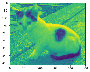
1 灰度图
# opencv读取的格式是BGR
# matplotlib读取的格式是RGB
import cv2
import numpy as np
import matplotlib.pyplot as plt
%matplotlib inline

img = cv2.imread("cat.jpg")
img_gray = cv2.cvtColor(img,cv2.COLOR_BGR2GRAY)
img_gray.shape
(414, 500)
cv2.imshow("img_gray",img_gray)
cv2.waitKey(0)
cv2.destroyAllWindows()
plt.imshow(img_gray)
<matplotlib.image.AxesImage at 0x1cc481f5128>
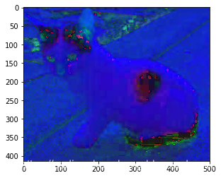
2 HSV
- H -色调(主波长)
- S -饱和度(纯度/颜色的阴影)
- V - 强度
hsv = cv2.cvtColor(img,cv2.COLOR_BGR2HSV)
cv2.imshow("hsv",hsv)
cv2.waitKey(0)
cv2.destroyAllWindows()
plt.imshow(hsv)
<matplotlib.image.AxesImage at 0x1cc34feada0>
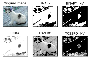
3 图像阈值
ret, dst = cv2.threshold(src, thresh, maxval, type)
-
src: 输入图,只能输入单通道图像,通常来说为灰度图
-
dst: 输出图
-
thresh: 阈值
-
maxval: 当像素值超过了阈值(或者小于阈值,根据type来决定),所赋予的值
-
type:二值化操作的类型,包含以下5种类型: cv2.THRESH_BINARY; cv2.THRESH_BINARY_INV; cv2.THRESH_TRUNC; cv2.THRESH_TOZERO;cv2.THRESH_TOZERO_INV
-
cv2.THRESH_BINARY 超过阈值部分取maxval(最大值),否则取0
-
cv2.THRESH_BINARY_INV THRESH_BINARY的反转
-
cv2.THRESH_TRUNC 大于阈值部分设为阈值,否则不变
-
cv2.THRESH_TOZERO 大于阈值部分不改变,否则设为0
-
cv2.THRESH_TOZERO_INV THRESH_TOZERO的反转
ret, thresh1 = cv2.threshold(img_gray, 127, 255, cv2.THRESH_BINARY)
ret, thresh2 = cv2.threshold(img_gray, 127, 255, cv2.THRESH_BINARY_INV)
ret, thresh3 = cv2.threshold(img_gray, 127, 255, cv2.THRESH_TRUNC)
ret, thresh4 = cv2.threshold(img_gray, 127, 255, cv2.THRESH_TOZERO)
ret, thresh5 = cv2.threshold(img_gray, 127, 255, cv2.THRESH_TOZERO_INV)

titles = ['Original Image', 'BINARY', 'BINARY_INV', 'TRUNC', 'TOZERO', 'TOZERO_INV']
images = [img, thresh1, thresh2, thresh3, thresh4, thresh5]

for i in range(6):
    plt.subplot(2, 3, i + 1), plt.imshow(images[i], 'gray')
    plt.title(titles[i])
    plt.xticks([]), plt.yticks([])
plt.show()
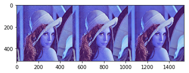
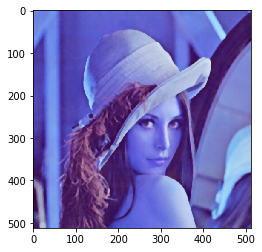
4 图像平滑
img = cv2.imread("lenaNoise.png")

cv2.imshow("img",img)
cv2.waitKey(0)
cv2.destroyAllWindows()

plt.imshow(img)
<matplotlib.image.AxesImage at 0x1cc44d79080>

均值滤波
- 简单的平均卷积操作
blur = cv2.blur(img,(3,3))

cv2.imshow("blur",blur)
cv2.waitKey(0)
cv2.destroyAllWindows()

plt.imshow(blur)
<matplotlib.image.AxesImage at 0x1cc35cbc748>

方框滤波
- 基本和均值一样,可以选择归一化
box = cv2.boxFilter(img,-1,(3,3), normalize=True)

cv2.imshow('box', box)
cv2.waitKey(0)
cv2.destroyAllWindows()

plt.imshow(box)
<matplotlib.image.AxesImage at 0x1cc48671400>

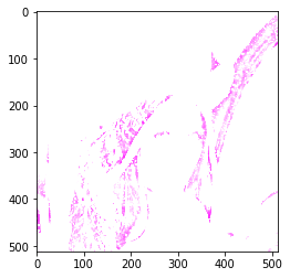
box = cv2.boxFilter(img,-1,(3,3), normalize=False)

cv2.imshow('box', box)
cv2.waitKey(0)
cv2.destroyAllWindows()

plt.imshow(box)
<matplotlib.image.AxesImage at 0x1cc44e33a90>
高斯滤波
- 高斯模糊的卷积核里的数值是满足高斯分布,相当于更重视中间的
aussian = cv2.GaussianBlur(img, (5, 5), 1)

cv2.imshow("aussian", aussian)
cv2.waitKey(0)
cv2.destroyAllWindows()

plt.imshow(aussian)
<matplotlib.image.AxesImage at 0x1cc35020f60>

中值滤波
median = cv2.medianBlur(img,5)

cv2.imshow("median", median)
cv2.waitKey(0)
cv2.destroyAllWindows()

plt.imshow(median)
<matplotlib.image.AxesImage at 0x1cc42c25b00>
# 展示所有的
res = np.hstack((blur,aussian,median))
cv2.imshow("median vs average",res)
cv2.waitKey(0)
cv2.destroyAllWindows()

plt.imshow(res)
<matplotlib.image.AxesImage at 0x1cc486ae470>