基础知识和详细版可以参考这个
https://blog.csdn.net/piaoxuezhong/article/details/78818572

代码老师没有细讲，还得自己悟和注释，浪费时间…

'''pylot使用rc配置文件来自定义图形的各种默认属性，称
之为rc配置或rc参数。通过rc参数可以修改默认的属性，
包括窗体大小、每英寸的点数、线条宽度、颜色、样式、坐标轴、坐标和网络属性、文本、字体等。
https://www.cnblogs.com/pacino12134/p/9776882.html'''
import numpy as np
import matplotlib.pyplot as plt

#cmap  https://blog.csdn.net/lanchunhui/article/details/66972783

plt.rcParams["figure.figsize"]=(10.0,8.0)
plt.rcParams["image.interpolation"]="nearest"
plt.rcParams["image.cmap"]="gray"

'''原来每次运行代码时设置相同的seed，则每次生成的随机数也相同，
如果不设置seed，则每次生成的随机数都会不一样。

np.linspace(start, stop, num=50, endpoint=True, retstep=False, dtype=None)

在规定的时间内，返回固定间隔的数据。他将返回“num”个等间距的样本，在区间[start, stop]中。其中，区间的结束端点可以被排除在外。
'''

np.random.seed(0)
N=100#number of points per class
D=2 #dimensioanlity 
K=3 #number of classes
X=np.zeros(N*D,K)
y=np.zeros(N*D,dtype="unit8")
for j in xrange(K):
    ix=range(N*j,N*(j+1))
    r=np.linspance(0.0,1,N)#radius
    t=np.linspance(j*4,(j+1)*4,N)+np.random.randn*(N)*0.2  #theta
    x[ix]=np.c_[r*np.sin(t),r*np.cos(t)]
    x[ix]=j
    '''ix: range(0, 100)
       ix: range(100, 200)
       ix: range(200, 300)'''
 #给300个点分类，每一百为一类，即[0，99]为0类，[100，199]为1类，[200,299]为2类   
W=0.01*np.random.randn(D,K)
b=np.zeros((1,k))

#some hyperparameters
step_size=1e-0
reg=1e-3 #regularization strength  还是加上了正则化惩罚项

#gradient descent loop
num_examples=X.shape[0]
# a.shape[0] #计算行数   https://www.jb51.net/article/111770.htm
for i in xrange(1000):
    scores=np.dot[X,W]+b
    exp_scores=np.exp(scores)#np.exp(B) : 求e的幂次方
    probs=exp_scores/np.sum(exp_scores,axis=1,keepdims=True)
    
    #compute the loss:average cross-entropy loss and regularization
    corect_logprobs=-np.log(probs[range(num_examples),y])
   # https://stackoverflow.com/questions/36158469/what-is-meaning-of-using-probsrange6-y

    data_loss=np.sum(corect_logprobs)/num_examples
    reg_loss=0.5*reg*np.sum(W*W)
    loss=data_loss+reg_loss
    
    if i%100==0:
        print("iteration %d:loss %f" %(i,loss))
        
     #compute the gradient on scores
    #反向传播计算梯度
    dscores=probs
    dscores[range(num_examples),y]-=1
    dscores/=num_examples
    
    #backpropate the gradient to the parameters(W,b)
    dW=np.dot(X.T,dscores)
    db=np.sum(dscores,axis=0,keepdims=True)
    dW+=reg*W   # don't forget the regularization gradient
    #其中，对W求导时，两边同乘 X.T。第三行dW加上了正则项（1/2*λ*W^2）部分对W的导数（λW）
    
    #perform a parameter
    
    W+=-step_size*dW
    b+=-step_size*db
    scores=np.dot(X,W)+b
predicted_class=np.argmax(scores,axis=1
print ('training accuracy: %.2f' % (np.mean(predicted_class == y))))

    
    
    

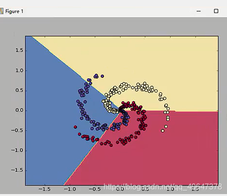
生成的数据集图像呈现

结果:可以看出效果不好，线性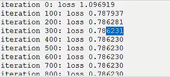
分成的三类

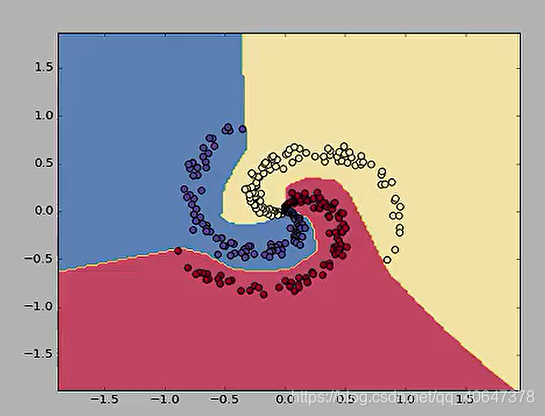
下面看神经网络的效果

#generate data
N = 100 # number of points per class
D = 2 # dimensionality
K = 3 # number of classes
import numpy as np
import matplotlib.pyplot as plt
X = np.zeros((N*K,D)) # data matrix (each row = single example)
y = np.zeros(N*K, dtype='uint8') # class labels
for j in range(K):
  ix = range(N*j,N*(j+1))
#  print("ix:",ix)
  r = np.linspace(0.0,1,N) # radius
  t = np.linspace(j*4,(j+1)*4,N) + np.random.randn(N)*0.2 # theta
  X[ix] = np.c_[r*np.sin(t), r*np.cos(t)]
#  print("X[ix]:",X[ix])
  y[ix] = j
# lets visualize the data:
plt.scatter(X[:, 0], X[:, 1], c=y, s=50)
#plt.scatter(X[:, 0], X[:, 1], c=y, s=40, cmap=plt.cm.Spectral)
plt.show()
 
# initialize parameters randomly
h = 100 # size of hidden layer
W = 0.01 * np.random.randn(D,h)
b = np.zeros((1,h))
W2 = 0.01 * np.random.randn(h,K)
b2 = np.zeros((1,K))
 
# some hyperparameters
step_size = 1e-0
reg = 1e-3 # regularization strength
 
# gradient descent loop
num_examples = X.shape[0]
for i in range(10000):
  
  # evaluate class scores, [N x K]
  hidden_layer = np.maximum(0, np.dot(X, W) + b) # note, ReLU activation
  scores = np.dot(hidden_layer, W2) + b2
  
  # compute the class probabilities
  exp_scores = np.exp(scores)
  probs = exp_scores / np.sum(exp_scores, axis=1, keepdims=True) # [N x K]
  
  # compute the loss: average cross-entropy loss and regularization
  corect_logprobs = -np.log(probs[range(num_examples),y])
  data_loss = np.sum(corect_logprobs)/num_examples
  reg_loss = 0.5*reg*np.sum(W*W) + 0.5*reg*np.sum(W2*W2)
  loss = data_loss + reg_loss
  if i % 1000 == 0:
    print ("iteration %d: loss %f" % (i, loss))
  
  # compute the gradient on scores
  dscores = probs
  dscores[range(num_examples),y] -= 1
  dscores /= num_examples
  
  # backpropate the gradient to the parameters
  # first backprop into parameters W2 and b2
  dW2 = np.dot(hidden_layer.T, dscores)
  db2 = np.sum(dscores, axis=0, keepdims=True)
  # next backprop into hidden layer
  dhidden = np.dot(dscores, W2.T)
  # backprop the ReLU non-linearity
  dhidden[hidden_layer <= 0] = 0
  # finally into W,b
  dW = np.dot(X.T, dhidden)
  db = np.sum(dhidden, axis=0, keepdims=True)
  
  # add regularization gradient contribution
  dW2 += reg * W2
  dW += reg * W
  
  # perform a parameter update
  W += -step_size * dW
  b += -step_size * db
  W2 += -step_size * dW2
  b2 += -step_size * db2
  
# evaluate training set accuracy
hidden_layer = np.maximum(0, np.dot(X, W) + b)
scores = np.dot(hidden_layer, W2) + b2
predicted_class = np.argmax(scores, axis=1)
print ('training accuracy: %.2f' % (np.mean(predicted_class == y)))
 
# plot the resulting classifier
h = 0.02
x_min, x_max = X[:, 0].min() - 1, X[:, 0].max() + 1
y_min, y_max = X[:, 1].min() - 1, X[:, 1].max() + 1
xx, yy = np.meshgrid(np.arange(x_min, x_max, h),
                     np.arange(y_min, y_max, h))
# np.meshgrid https://blog.csdn.net/starter_____/article/details/79176413                     
Z = np.dot(np.maximum(0, np.dot(np.c_[xx.ravel(), yy.ravel()], W) + b), W2) + b2
Z = np.argmax(Z, axis=1)
Z = Z.reshape(xx.shape)
fig = plt.figure()
plt.contourf(xx, yy, Z, cmap=plt.cm.Spectral, alpha=0.8)
plt.scatter(X[:, 0], X[:, 1], c=y, s=40)
plt.xlim(xx.min(), xx.max())
plt.ylim(yy.min(), yy.max())
plt.show()

结果

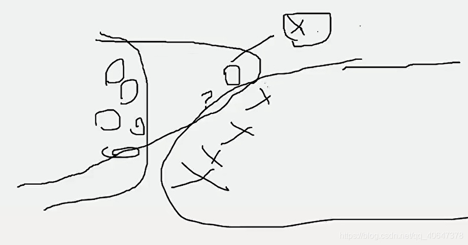
为了这一个点，神经网络可能需要多走很多步，过拟合