文章目录
注:所将可能是python2演示的,而与Python3有区别,要注意。
一、pandas 索引

序列以及二维数组的索引
#np.random.rand(d0,d1,d2……dn)
注:使用方法与np.random.randn()函数相同
作用:
通过本函数可以返回一个或一组服从“0~1”均匀分布的随机样本值。随机样本取值范围是[0,1),不包括1。
应用:在深度学习的Dropout正则化方法中,可以用于生成dropout随机向量(dl),例如(keep_prob表示保留神经元的比例):dl = np.random.rand(al.shape[0],al.shape[1]) < keep_prob
s1=pd.Series(np.random.rand(5),index=['a','b','c','d','e'])

#1查看Series序列索引
print(s1.index)
#2为索引赋一个名字
s1.index.name='alpha'
print(s1)
结果:
D:\ProgramData\Anaconda3\python.exe D:/numpy-kexue/03.py
Index(['a', 'b', 'c', 'd', 'e'], dtype='object')
alpha
a    0.334112
b    0.074574
c    0.689593
d    0.448733
e    0.157336
dtype: float64

Process finished with exit code 0


data3=pd.DataFrame(np.random.randn(4,3),columns=['one','two','three'])
print(data3)
#1二维数组获取行索引
print(data3.index)
#2二维数组获取列索引
print(data3.columns)
#3为行列索引起名字
data3.index.name='row'
data3.columns.name='col'
print(data3)
#4pandas中内置了很多索引的类,如RangeIndex,Index这里以python3为例,视频中是Python2,有些区别
#查询pandas中内置的索引类
结果:
D:\ProgramData\Anaconda3\python.exe D:/numpy-kexue/03.py
        one       two     three
0 -0.300068  0.107822 -0.461084
1  0.071834 -0.927457  0.323366
2 -0.103444 -0.157807 -2.089129
3  0.752966 -1.488562  0.781543
RangeIndex(start=0, stop=4, step=1)
Index(['one', 'two', 'three'], dtype='object')
col       one       two     three
row
0   -0.300068  0.107822 -0.461084
1    0.071834 -0.927457  0.323366
2   -0.103444 -0.157807 -2.089129
3    0.752966 -1.488562  0.781543

Process finished with exit code 0
重复索引
s1=pd.Series(np.arange(6),index=['a','b','c','b','d','a'])
print(s1)
#1重复索引a有两个值,返回Series
print(s1['a'])
#2未重复索引返回是一个标量数据
print(s1['c'])
#3判断是否有重复索引
print(s1.index.is_unique)#False,即有重复索引
#4返回唯一索引
print(s1.index.unique())
#5对有重复索引的数据进行清洗,与业务有关,有时只需要保留第一个重复索引值,有时要把重复索引值加起来,或求平均
print(s1.groupby(s1.index).sum())#根据索引分组之后求和来聚合,求平均mean()
结果:
D:\ProgramData\Anaconda3\python.exe D:/numpy-kexue/03.py
a    0
b    1
c    2
b    3
d    4
a    5
dtype: int32
a    0
a    5
dtype: int32
2
False
Index(['a', 'b', 'c', 'd'], dtype='object')
a    5
b    4
c    2
d    4
dtype: int32

Process finished with exit code 0
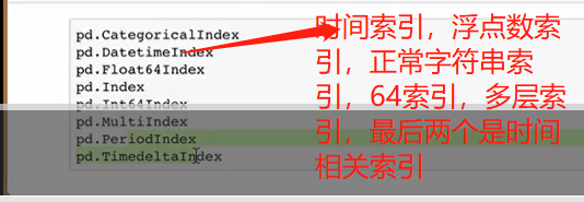
多层索引
MultiIndex多层索引类
注:可以将更高维度数据用二维数据表示。行两个索引,列一个索引就表示三维数组,二维数组可读性比高维度高。
例如:股票行索引日期与股票代码,列索引:股票开盘价,收盘价,成交量来表示。
#1创建多级索引
a=[['a','a','a','b','b','c','c'],[1,2,3,1,2,2,3]]
#将列表用zip组装成内层为元组形式。以下两种形式等价
# t=list(zip(*a))#这种形式与a=zip(['a','a','a','b','b','c','c'],[1,2,3,1,2,2,3])
# #结果中就是两个元组中的元素两两依次组合[('a', 1), ('a', 2), ('a', 3), ('b', 1), ('b', 2), ('c', 2), ('c', 3)]
# print(t)#print(list(a))等价
t=list(zip(a))
print(*a)#['a', 'a', 'a', 'b', 'b', 'c', 'c'] [1, 2, 3, 1, 2, 2, 3]解包后发现就是两个列表,在用zip函数进行合并时就是每一个列表中取一个组成元组。
#所以刚才的等价,因为后者a=zip(['a','a','a','b','b','c','c'],[1,2,3,1,2,2,3])就是直接传进两个列表了,所以不需要解包了。
# t=list(zip(a))print(t)#这种没有解包,直接将a=[['a','a','a','b','b','c','c'],[1,2,3,1,2,2,3]]大列表进行合并所以就只有一个列表
#即整体取第一个元素即['a', 'a', 'a', 'b', 'b', 'c', 'c']因为没第二个列表元素,但又要是元组,所以加了个逗号;将列表中第二部分也取出来,变为元组加逗号。
# 所以结果才为[   (['a', 'a', 'a', 'b', 'b', 'c', 'c'],)    ,    ([1, 2, 3, 1, 2, 2, 3],)     ]
Series多级索引
#1创建多级索引
a=[['a','a','a','b','b','c','c'],[1,2,3,1,2,2,3]]
#将列表用zip组装成内层为元组形式。以下两种形式等价
# t=list(zip(*a))#这种形式与a=zip(['a','a','a','b','b','c','c'],[1,2,3,1,2,2,3])
# #结果中就是两个元组中的元素两两依次组合[('a', 1), ('a', 2), ('a', 3), ('b', 1), ('b', 2), ('c', 2), ('c', 3)]
# print(t)#print(list(a))等价
t=list(zip(*a))
print(t)#可以用这个数组结果创建多级索引了。

#2创建多级索引,并起名字
inde=pd.MultiIndex.from_tuples(t,names=['level1','level2'])
print(inde)
#3有了多层索引就可以创建Series或DataFrame了,7个索引就有7个数据
s=pd.Series(np.random.rand(7),index=inde)
print(s)
#3选取1级所以为b的所有元素出来
print(s['b'])
#4选取1级所以为b与c的所有元素出来
print(s['b':'c'])
#5用列表选取1级所以为a与c的所有元素出来
print(s[['a','c']])
#6 1级索引任意,2级索引为2的出来
print(s[:,2])
结果:
D:\ProgramData\Anaconda3\python.exe D:/numpy-kexue/03.py
[('a', 1), ('a', 2), ('a', 3), ('b', 1), ('b', 2), ('c', 2), ('c', 3)]
MultiIndex(levels=[['a', 'b', 'c'], [1, 2, 3]],
           codes=[[0, 0, 0, 1, 1, 2, 2], [0, 1, 2, 0, 1, 1, 2]],
           names=['level1', 'level2'])
level1  level2
a       1         0.567812
        2         0.936409
        3         0.194581
b       1         0.090835
        2         0.490026
c       2         0.877824
        3         0.796039
dtype: float64
level2
1    0.090835
2    0.490026
dtype: float64
level1  level2
b       1         0.090835
        2         0.490026
c       2         0.877824
        3         0.796039
dtype: float64
level1  level2
a       1         0.567812
        2         0.936409
        3         0.194581
c       2         0.877824
        3         0.796039
dtype: float64
level1
a    0.936409
b    0.490026
c    0.877824
dtype: float64

Process finished with exit code 0
DataFrame多级索引
#1直接创建DataFrame的多级索引,行列索引各两层,并为行列的每层索引命名
#index=[['a','a','b','b'],[1,2,1,2]]这种就是列表套列表的,即2层索引就是内层第一个列表为一个索引,内层第二个列表也是一个索引
da1 = pd.DataFrame(np.random.randint(1,10,(4,3)),  index=[['a','a','b','b'],[1,2,1,2]],
                   columns=[['one','one','two'],['blue','red','blue']])
# 2并为行列的每层索引命名
da1.index.names=['row-1','row-2']
da1.columns.names=['col-1','col-2']
print(da1)
#3选取1级行索引a,其实也是一个DataFrame
print(type(da1.loc['a']))#<class 'pandas.core.frame.DataFrame'>#
# pandas.core.frame.DataFrame 就代表了我们这里DataFrame来自frame模块,而frame模块是属于core模块的,同时pandas包又是由core模块等组成。
# Pandas有两个主要的数据结构:Series和DataFrame都是这样的
#Pandas 的数据结构 DataFrame 即数据集的常用方法
print(da1.loc['a'])
#4选取1级索引为a,2级索引为1的,就是一个二级索引的序列
print(da1.loc['a',1 ])
print(da1.loc['a',1 ].index)
#二级索引,codes=[[0, 0, 1], [0, 1, 0]],就是1级索引one为0 two为1;2级索引blue为0,red为1;
# 在[['one','one','two'],['blue','red','blue']]中的位置所以就是[[0, 0, 1], [0, 1, 0]]了
结果:
D:\ProgramData\Anaconda3\python.exe D:/numpy-kexue/03.py
col-1        one      two
col-2       blue red blue
row-1 row-2
a     1        9   6    4
      2        1   8    3
b     1        1   2    3
      2        4   6    3
<class 'pandas.core.frame.DataFrame'>
col-1  one      two
col-2 blue red blue
row-2
1        9   6    4
2        1   8    3
col-1  col-2
one    blue     9
       red      6
two    blue     4
Name: (a, 1), dtype: int32
MultiIndex(levels=[['one', 'two'], ['blue', 'red']],
           codes=[[0, 0, 1], [0, 1, 0]],
           names=['col-1', 'col-2'])
索引的交换
#1直接创建DataFrame的多级索引,行列索引各两层,并为行列的每层索引命名
#index=[['a','a','b','b'],[1,2,1,2]]这种就是列表套列表的,即2层索引就是内层第一个列表为一个索引,内层第二个列表也是一个索引
da1 = pd.DataFrame(np.random.randint(1,10,(4,3)),  index=[['a','a','b','b'],[1,2,1,2]],
                   columns=[['one','one','two'],['blue','red','blue']])
# 2并为行列的每层索引命名
da1.index.names=['row-1','row-2']
da1.columns.names=['col-1','col-2']
print(da1)
#3将行索引的两个交换,原来da1不变
da2=da1.swaplevel('row-1','row-2')
print(da1)
print(da2)
#4对交换后的索引即da2按照1级索引进行排序,所以为0即1级索引
# da2.sort_level(0)
# print(da2)
#5多级索引下进行统计
#根据1级索引求和即0,即1级索引以后的值都加起来,或根据二级索引求和即(level=1)
print(da1.sum(level=0))
结果:
D:\ProgramData\Anaconda3\python.exe D:/numpy-kexue/03.py
col-1        one      two
col-2       blue red blue
row-1 row-2
a     1        1   7    5
      2        9   9    7
b     1        4   8    2
      2        6   8    3
col-1        one      two
col-2       blue red blue
row-1 row-2
a     1        1   7    5
      2        9   9    7
b     1        4   8    2
      2        6   8    3
col-1        one      two
col-2       blue red blue
row-2 row-1
1     a        1   7    5
2     a        9   9    7
1     b        4   8    2
2     b        6   8    3
col-1  one      two
col-2 blue red blue
row-1
a       10  16   12
b       10  16    5

Process finished with exit code 0
文件读取创建多级索引
#一般我们会从文件中读取DataFrame出来,将里面有些列设置成索引,这样来构成多级索引的DataFrame,而不是一个一个索引写麻烦。
#字典直接将键作为列索引了,行默认索引;
#1如从文件中读取出来假如为下边的这个DataFrame
df1=pd.DataFrame({'a':range(7),
                  'b':range(7,0,-1),
                  'c':['one','one','one','two','two','two','two'],
                  'd':[0,1,2,0,1,2,3]})
print(df1)
#2将某些列设置成索引值
print(df1.set_index('c'))
#3将c与d都作为索引生成2级索引
df2=df1.set_index(['c','d'])
print(df1.set_index(['c','d']))
#4将二级索引的df2再变回去为原来的df1形式,只不过a b c d 顺序有变化,其他一样
df3=df2.reset_index()
print(df3)
#4将df3根据列索引排序就真正回到df1了。
print(df3.sort_index('columns'))
print(df2.reset_index().sort_index('columns')==df1)
#发现都是true所以说明df2.reset_index().sort_index('columns')与df1一样了。
#上面的df3我们分两步进行,也可以一步转到df1如:df2.reset_index().sort_index('columns')
结果:
D:\ProgramData\Anaconda3\python.exe D:/numpy-kexue/03.py
   a  b    c  d
0  0  7  one  0
1  1  6  one  1
2  2  5  one  2
3  3  4  two  0
4  4  3  two  1
5  5  2  two  2
6  6  1  two  3
     a  b  d
c
one  0  7  0
one  1  6  1
one  2  5  2
two  3  4  0
two  4  3  1
two  5  2  2
two  6  1  3
       a  b
c   d
one 0  0  7
    1  1  6
    2  2  5
two 0  3  4
    1  4  3
    2  5  2
    3  6  1
     c  d  a  b
0  one  0  0  7
1  one  1  1  6
2  one  2  2  5
3  two  0  3  4
4  two  1  4  3
5  two  2  5  2
6  two  3  6  1
   a  b    c  d
0  0  7  one  0
1  1  6  one  1
2  2  5  one  2
3  3  4  two  0
4  4  3  two  1
5  5  2  two  2
6  6  1  two  3
      a     b     c     d
0  True  True  True  True
1  True  True  True  True
2  True  True  True  True
3  True  True  True  True
4  True  True  True  True
5  True  True  True  True
6  True  True  True  True

Process finished with exit code 0
二、pandas 分组运算
总图:

分组原理:

第一部分分组

df1=pd.DataFrame({'key1':['a','a','b','b','a',],
                  'key2':['one','two','one','two','one'],
                  'data1':np.random.randint(1,10,5),
                  'data2':np.random.randint(1,10,5)})
print(df1)
print(df1['data1'])
df3=df1['data1'].groupby(df1['key1'])
print(df3)#<pandas.core.groupby.generic.SeriesGroupBy object at 0x000002531D8D1C50>#是一个分组对象了。
#1取出'data1'这一列并根据key1为键进行分组,用求平均聚合,用不重复的key1为索引输出结果即可。
df2=df1['data1'].groupby(df1['key1']).mean()
print(df2)
#2分组的键索引不一定必须是df1中的某一列,也可以定义
key=[1,2,1,1,2]
df4=df1['data1'].groupby(key).mean()
print(df4)
#3将data1这一列数据生成有多层索引的Series序列,即先根据key1分组,之后分完后再根据key2分组
df5=df1['data1'].groupby([df1['key1'],df1['key2']]).mean()
print(df5)
#4看上一步分组后的个数
print(df1['data1'].groupby([df1['key1'],df1['key2']]).size())
#5直接对整个数组df1分组,,因为key2不是数字,所以分组计算时就把他扔掉了。
df6=df1.groupby('key1').sum()
print(df6)
#6 df6又是数组,所以可以只看data1结果
df7=df1.groupby('key1').sum()['data1']
print(df7)
#7对整个数组指定多层索引进行分组,之后取data1数据
df8=df1.groupby(['key1','key2']).sum()['data1']
print(df8)
#8将df8转化为datafram格式,即行与列索引
df9=df8.unstack()
print(df9)
#9pandas分组groupby支持python的迭代器协议的,所以直接可以用for迭代
for name ,group in df1.groupby('key1'):#每次迭代返回分组的名字与对应数据
    print(name)
    print(group)
#10groupby支持python的迭代器协议的,也可以直接转化为列表或字典
#a=list(df1.groupby('key1'))#结果是列表中套的元组作为元素
#print(a)
#b=dict(list(df1.groupby('key1')))
#print(b)#转化为字典了。
a=dict(list(df1.groupby('key1')))
print(a)
print(a['a'])#获取键a对应大的数据

#11以上都是按照axis=0方向分组的,也可以按照列axis=1的方向进行分组
#看一下各列数据类型
print(df1.dtypes)#df1.dtypes就是序列即<class 'pandas.core.series.Series'>
print(df1.dtypes.value_counts())
print(type(df1.dtypes))
#12 按照列方向分组,即按照df1.dtypes的序列值int32与object进行分成2组即可,发现求和时对应字符串连接起来了。
df10=df1.groupby(df1.dtypes,axis=1).sum()
print(df10)
结果:
D:\ProgramData\Anaconda3\python.exe D:/numpy-kexue/03.py
  key1 key2  data1  data2
0    a  one      8      4
1    a  two      2      6
2    b  one      3      5
3    b  two      5      1
4    a  one      9      1
0    8
1    2
2    3
3    5
4    9
Name: data1, dtype: int32
<pandas.core.groupby.generic.SeriesGroupBy object at 0x000001B971F1AFD0>
key1
a    6.333333
b    4.000000
Name: data1, dtype: float64
1    5.333333
2    5.500000
Name: data1, dtype: float64
key1  key2
a     one     8.5
      two     2.0
b     one     3.0
      two     5.0
Name: data1, dtype: float64
key1  key2
a     one     2
      two     1
b     one     1
      two     1
Name: data1, dtype: int64
      data1  data2
key1
a        19     11
b         8      6
key1
a    19
b     8
Name: data1, dtype: int32
key1  key2
a     one     17
      two      2
b     one      3
      two      5
Name: data1, dtype: int32
key2  one  two
key1
a      17    2
b       3    5
a
  key1 key2  data1  data2
0    a  one      8      4
1    a  two      2      6
4    a  one      9      1
b
  key1 key2  data1  data2
2    b  one      3      5
3    b  two      5      1
{'a':   key1 key2  data1  data2
0    a  one      8      4
1    a  two      2      6
4    a  one      9      1, 'b':   key1 key2  data1  data2
2    b  one      3      5
3    b  two      5      1}
  key1 key2  data1  data2
0    a  one      8      4
1    a  two      2      6
4    a  one      9      1
key1     object
key2     object
data1     int32
data2     int32
dtype: object
int32     2
object    2
dtype: int64
<class 'pandas.core.series.Series'>
   int32 object
0     12   aone
1      8   atwo
2      8   bone
3      6   btwo
4     10   aone

Process finished with exit code 0
通过字典进行分组
df1=pd.DataFrame(np.random.randint(1,10,(5,5)),
                columns=['a','b','c','d','e'],
                 index=['Alice','Bob','Candy','Dark','Emily'])
#将两个元素变为NaN,在Python中用iloc与loc,不要用python2中的ix会警告
# df1.ix[1,1:3]=np.NaN
df1.loc['Bob','b':'c']=np.NaN
print(df1)
#1说明非数字在分组中的情况处理,创建一个字典作为分组的key,将a这一列名称映射到red,其他依次映射
mapp={'a':'red','b':'red','c':'blue','d':'orange','e':'blue'}
#2分组时,df1按照字典映射关系进行分组
grou=df1.groupby(mapp,axis=1)#因为映射关系根据列名称来的,所以写成列按照列来分组
#对分好的组进行求和,发现NaN作为0处理了。
df2=grou.sum()
print(df2)
#3查看分组后的各个数量,blue为2列
print(grou.size())
#4查看对于每一个分组后,如blue对应的行标签Alice 的数目为2,其他类似。且NaN不计入数目
print(grou.count())
结果:
D:\ProgramData\Anaconda3\python.exe D:/numpy-kexue/03.py
       a    b    c  d  e
Alice  2  4.0  4.0  7  8
Bob    5  NaN  NaN  9  9
Candy  7  2.0  1.0  8  2
Dark   9  3.0  5.0  4  1
Emily  5  5.0  6.0  4  4
       blue  orange   red
Alice  12.0     7.0   6.0
Bob     9.0     9.0   5.0
Candy   3.0     8.0   9.0
Dark    6.0     4.0  12.0
Emily  10.0     4.0  10.0
blue      2
orange    1
red       2
dtype: int64
       blue  orange  red
Alice     2       1    2
Bob       1       1    1
Candy     2       1    2
Dark      2       1    2
Emily     2       1    2

Process finished with exit code 0
通过函数进行分组
df1=pd.DataFrame(np.random.randint(1,10,(5,5)),
                columns=['a','b','c','d','e'],
                 index=['Alice','Bob','Candy','Dark','Emily'])
print(df1)
#1通过函数分组,函数参数为分组时候要计算的索引名字,就是根据函数返回值进行分组的。
# def groupky(idx):
#     print(idx)#通过打印每一次的分组标签,可以看到默认是按照行进行分组的。所以这句话将每一行索引打出来
#     return  idx
# df2=df1.groupby(groupky)
# print(df2)
# print(df2.size())#按照行分组,所以行索引没有重复的,所以每一个分组都只有一组数据。

# #2
# def groupky(idx):
#     print(idx)#通过打印每一次的分组标签,可以看到默认是按照行进行分组的。所以这句话将每一行索引打出来
#     return  len(idx)#分组返回按照字母的长度分组,如Bob有三个字符即3为一组:
#     # 数量有1个;Candy,Alice,Emily有5个字符,所以5个字符的分组数目为3个。
# df2=df1.groupby(groupky)
# print(df2)
# print(df2.size())#按照行分组,所以行索引没有重复的,所以每一个分组都只有一组数据。

#3  上面2的按照行标签的字符个数分组方式,效果一样,其最简单的写法为:因为len就是函数,且默认又是按照行索引分组
df2=df1.groupby(len).size()
print(df2)
print(df1.groupby(len).sum())#因为字符个数为5的有三个数目,对应相加,其他2个组就一组,所以不动
D:\ProgramData\Anaconda3\python.exe D:/numpy-kexue/03.py
       a  b  c  d  e
Alice  9  9  7  8  9
Bob    2  3  7  6  8
Candy  8  3  4  3  9
Dark   4  8  6  5  3
Emily  4  8  2  1  9
3    1
4    1
5    3
dtype: int64
    a   b   c   d   e
3   2   3   7   6   8
4   4   8   6   5   3
5  21  20  13  12  27

Process finished with exit code 0
多级索引分组情况
#1创建一个多级索引,列索引两层,行索引默认
colunm=pd.MultiIndex.from_arrays([['China','USA','China','USA','China'],
                                  ['A','A','B','C','B']],names=['country','index'])
#注意这里不用from_tuples因为1内层不是元组形式
# 2因为用两个索引,所以列表的内层必须是元组形式,即[('a', 1), ('a', 2), ('a', 3), ('b', 1), ('b', 2), ('c', 2), ('c', 3)]
# 且每个元组中个数必须保证是2个如('a', 1),而内层元组个数可以多个。('a', 1)、('a', 3),这多个元组
#因为不满足元组条件所以用的是数组创建的多层索引from_arrays,列表中的各个小列表作为一个索引
#2查看多级索引
print(colunm)
df1=pd.DataFrame(np.random.randint(1,10,(5,5)),
                columns=colunm)
print(df1)

#3多级索引分组时,可以根据索引级别进行分组。
df2=df1.groupby(level='country',axis=1)#根据country分组是列索引,所以必须指定按照列分组,因为默认行索引没这个。
print(df2)
print(df2.sum())
#4按照index分组
df3=df1.groupby(level='index',axis=1)#根据index分组是列索引,所以必须指定按照列分组,因为默认行索引没这个。
print(df3)
print(df3.sum())
结果:
D:\ProgramData\Anaconda3\python.exe D:/numpy-kexue/03.py
MultiIndex(levels=[['China', 'USA'], ['A', 'B', 'C']],
           codes=[[0, 1, 0, 1, 0], [0, 0, 1, 2, 1]],
           names=['country', 'index'])
country China USA China USA China
index       A   A     B   C     B
0           9   4     8   6     4
1           2   4     9   6     9
2           7   7     6   1     1
3           6   6     8   4     9
4           4   7     5   8     8
<pandas.core.groupby.generic.DataFrameGroupBy object at 0x000001EB8F7D3D30>
country  China  USA
0           21   10
1           20   10
2           14    8
3           23   10
4           17   15
<pandas.core.groupby.generic.DataFrameGroupBy object at 0x000001EB8E0D0978>
index   A   B  C
0      13  12  6
1       6  18  6
2      14   7  1
3      12  17  4
4      11  13  8

Process finished with exit code 0
三、聚合运算
注:分组完后的数据进行计算即为聚合

内置聚合函数
df1=pd.DataFrame({'key1':['a','a','b','b','a',],
                  'key2':['one','two','one','two','one'],
                  'data1':np.random.randint(1,10,5),
                  'data2':np.random.randint(1,10,5)})
print(df1)
#1内置求和函数聚合,以及平均值mean,最小值min,最大值max,以及describe就是会对每个分组用一系列的内置函数进行聚合
print(df1.groupby('key1').sum())
自定义聚合函数
df1=pd.DataFrame({'key1':['a','a','b','b','a',],
                  'key2':['one','two','one','two','one'],
                  'data1':np.random.randint(1,10,5),
                  'data2':np.random.randint(1,10,5)})
print(df1)
df2=df1.groupby('key1')
#1自定义一个聚合函数最大值减去最小值
def  man(s):
    print(type(s))#聚合函数中的参数s就是逐个索引对应的记录。类型就是series,即每次
    # print(s)#类型就是series,即每次都是返回一个分组的对应数据
    return  s.max()-s.min()
#2用分组后的agg函数调用自定义函数进行聚合,将分好组的数据按照聚合函数进行计算了。
print(df2.agg(man))
#3将分组进行多个聚合函数运算一并返回
df3=df2.agg(['std','mean','sum',man])#标准差,平均值,求和,波动幅度即自定义的函数
print(df3)
#4自定义函数默认用函数名称作为分组聚合后的列名称,改列名称range作为聚合后的名字,执行man函数
df4=df2.agg(['std','mean','sum',('range',man)])
print(df4)
#5需求对于不同的列聚合函数不同,如对分组后的data1求平均,data2求和
#创建个字典
d={'data1':'mean',
   'data2':'sum'}
df5=df2.agg(d)
print(df5)
#6每一列聚合函数可以多个,分组后的索引就是key1的值
b={'data1':['mean',('range',man)],
   'data2':'sum'}
df6=df2.agg(b)
print(df6)
#7将分组后的索引值key1作为一列值,而不是索引
df7=df2.agg(b).reset_index()
print(df7)
#8对于7的简便方法,即在分组时候就默认让key1值不作为索引
df8=df1.groupby('key1',as_index=False).agg(b)
print(df8)
结果:
D:\ProgramData\Anaconda3\python.exe D:/numpy-kexue/03.py
  key1 key2  data1  data2
0    a  one      1      8
1    a  two      4      6
2    b  one      5      4
3    b  two      7      6
4    a  one      8      7
<class 'pandas.core.series.Series'>
<class 'pandas.core.series.Series'>
<class 'pandas.core.series.Series'>
<class 'pandas.core.series.Series'>
<class 'pandas.core.series.Series'>
<class 'pandas.core.series.Series'>
<class 'pandas.core.series.Series'>
<class 'pandas.core.series.Series'>
      data1  data2
key1
a         7      2
b         2      2
<class 'pandas.core.series.Series'>
<class 'pandas.core.series.Series'>
<class 'pandas.core.series.Series'>
<class 'pandas.core.series.Series'>
         data1                       data2
           std      mean sum man       std mean sum man
key1
a     3.511885  4.333333  13   7  1.000000    7  21   2
b     1.414214  6.000000  12   2  1.414214    5  10   2
<class 'pandas.core.series.Series'>
<class 'pandas.core.series.Series'>
<class 'pandas.core.series.Series'>
<class 'pandas.core.series.Series'>
         data1                         data2
           std      mean sum range       std mean sum range
key1
a     3.511885  4.333333  13     7  1.000000    7  21     2
b     1.414214  6.000000  12     2  1.414214    5  10     2
         data1  data2
key1
a     4.333333     21
b     6.000000     10
<class 'pandas.core.series.Series'>
<class 'pandas.core.series.Series'>
         data1       data2
          mean range   sum
key1
a     4.333333     7    21
b     6.000000     2    10
<class 'pandas.core.series.Series'>
<class 'pandas.core.series.Series'>
  key1     data1       data2
            mean range   sum
0    a  4.333333     7    21
1    b  6.000000     2    10
<class 'pandas.core.series.Series'>
<class 'pandas.core.series.Series'>
  key1     data1       data2
            mean range   sum
0    a  4.333333     7    21
1    b  6.000000     2    10

Process finished with exit code 0
分组聚合高级方法
df1=pd.DataFrame({'key1':['a','a','b','b','a',],
                  'key2':['one','two','one','two','one'],
                  'data1':np.random.randint(1,10,5),
                  'data2':np.random.randint(1,10,5)})
print(df1)
#1根据key1分组,并对data1,data2求平均再补两列,且索引也应该是0-4
#传统方法,复杂
#2先根据key1分组求平均
df2=df1.groupby('key1').mean()
print(df2)
#此时列只有2个元素,且也要将标签改一下。
df3=df2.add_prefix('mean_')
print(df3)#将列标签改了一下,都加上mean_了。
#将df3合并到df1之后,根据key1对应合并,根据df1的行标签进行对应合并,即True,否则报错
df4=pd.merge(df1,df3,left_on='key1',right_index=True )
print(df4)

#3简便的方法来合并两个表,分组根据平均值转化,j
df5=df1.groupby('key1').transform(np.mean)
print(df5)#转化为与原df1一样的结构大小
#重命名列名字
df6=df5.add_prefix('mean_')
print(df6)
#4合并两个表,即将df1增加两列为df6的列标签,值为df6
df1[df6.columns]=df6
print(df1)
结果:
D:\ProgramData\Anaconda3\python.exe D:/numpy-kexue/03.py
  key1 key2  data1  data2
0    a  one      3      8
1    a  two      8      3
2    b  one      8      1
3    b  two      4      4
4    a  one      1      3
      data1     data2
key1
a       4.0  4.666667
b       6.0  2.500000
      mean_data1  mean_data2
key1
a            4.0    4.666667
b            6.0    2.500000
  key1 key2  data1  data2  mean_data1  mean_data2
0    a  one      3      8         4.0    4.666667
1    a  two      8      3         4.0    4.666667
4    a  one      1      3         4.0    4.666667
2    b  one      8      1         6.0    2.500000
3    b  two      4      4         6.0    2.500000
   data1     data2
0      4  4.666667
1      4  4.666667
2      6  2.500000
3      6  2.500000
4      4  4.666667
   mean_data1  mean_data2
0           4    4.666667
1           4    4.666667
2           6    2.500000
3           6    2.500000
4           4    4.666667
  key1 key2  data1  data2  mean_data1  mean_data2
0    a  one      3      8           4    4.666667
1    a  two      8      3           4    4.666667
2    b  one      8      1           6    2.500000
3    b  two      4      4           6    2.500000
4    a  one      1      3           4    4.666667

Process finished with exit code 0
用自定义函数调用transform
df1=pd.DataFrame(np.random.randint(1,10,(5,5)),
                columns=['a','b','c','d','e'],
                 index=['Alice','Bob','Candy','Dark','Emily'])
print(df1)
#自定义一个函数
def dmean(s):#用每个分组的数据减去平均值。
    return  s-s.mean()
key=['one','one','two','one','two']
#根据key分组,并用transform传入自定义的函数
df2=df1.groupby(key).transform(dmean)
print(df2)#因为分组的key是['one','one','two','one','two'],即0 1 3行为一组,2与4即two这两行一组
#所以对于0.66667算式:因为0 1 3行为一组,所以对于a就是8,9,5平均值为7.333  所以用8-7.333为0.6667  9-7.33=1.6667
结果:
D:\ProgramData\Anaconda3\python.exe D:/numpy-kexue/03.py
       a  b  c  d  e
Alice  8  9  8  1  7
Bob    9  1  6  7  1
Candy  9  2  9  5  2
Dark   5  6  4  1  4
Emily  1  3  3  9  2
              a         b    c    d    e
Alice  0.666667  3.666667  2.0 -2.0  3.0
Bob    1.666667 -4.333333  0.0  4.0 -3.0
Candy  4.000000 -0.500000  3.0 -2.0  0.0
Dark  -2.333333  0.666667 -2.0 -2.0  0.0
Emily -4.000000  0.500000 -3.0  2.0  0.0

Process finished with exit code 0
df1=pd.DataFrame(np.random.randint(1,10,(5,5)),
                columns=['a','b','c','d','e'],
                 index=['Alice','Bob','Candy','Dark','Emily'])
print(df1)
#自定义一个函数
def dmean(s):#用每个分组的数据减去平均值。
    return  s-s.mean()
key=['one','one','two','one','two']
#根据key分组,并用transform传入自定义的函数
df2=df1.groupby(key).transform(dmean)
print(df2)#因为分组的key是['one','one','two','one','two'],即0 1 3行为一组,2与4即two这两行一组
#所以对于0.66667算式:因为0 1 3行为一组,所以对于a就是8,9,5平均值为7.333  所以用8-7.333为0.6667  9-7.33=1.6667
#因为df2已经是各个分组数据减去平均值了,即在平均值附近波动,在求平均值就是0
print(df2.groupby(key).mean( ))#结果中由于浮点数所以约为0的。
结果:
D:\ProgramData\Anaconda3\python.exe D:/numpy-kexue/03.py
       a  b  c  d  e
Alice  1  5  9  5  6
Bob    1  1  3  7  8
Candy  3  9  6  8  3
Dark   9  9  9  8  1
Emily  4  2  4  5  1
              a    b    c         d    e
Alice -2.666667  0.0  2.0 -1.666667  1.0
Bob   -2.666667 -4.0 -4.0  0.333333  3.0
Candy -0.500000  3.5  1.0  1.500000  1.0
Dark   5.333333  4.0  2.0  1.333333 -4.0
Emily  0.500000 -3.5 -1.0 -1.500000 -1.0
                a    b    c             d    e
one  2.960595e-16  0.0  0.0 -2.960595e-16  0.0
two  0.000000e+00  0.0  0.0  0.000000e+00  0.0

Process finished with exit code 0
df1=pd.DataFrame({'key1':['a','a','b','b','a','a','a','b','b','a'],
                  'key2':['one','two','one','two','one','one','two','one','two','one'],
                  'data1':np.random.randint(1,10,10),
                  'data2':np.random.randint(1,10,10)})
print(df1)
#1定义一个函数,参数分组g,输出2行,排列名称默认叫data1
def  top(g, n=2, column='data1'):
    return g.sort_values(by=column,ascending=False)[:n]#对分组排序,默认输出前n行
print(top(df1))#会根据data1排序,输出按照data1排序后的最大的前2行
print(top(df1,n=3))#输出前3行
#2 分组后调用apply函数输出分组后按照data1排序后的最大的前2行
df3=df1.groupby('key1').apply(top)#分组后,将分组后的各组数据给apply函数分别进行函数top运算
print(df3)
#3
df4=df1.groupby('key1').apply(top,n=3,column='data2')#根据data2排序
print(df4)
结果:
D:\ProgramData\Anaconda3\python.exe D:/numpy-kexue/03.py
  key1 key2  data1  data2
0    a  one      8      2
1    a  two      2      4
2    b  one      2      9
3    b  two      3      8
4    a  one      3      5
5    a  one      2      3
6    a  two      4      7
7    b  one      5      9
8    b  two      5      8
9    a  one      6      6
  key1 key2  data1  data2
0    a  one      8      2
9    a  one      6      6
  key1 key2  data1  data2
0    a  one      8      2
9    a  one      6      6
7    b  one      5      9
       key1 key2  data1  data2
key1
a    0    a  one      8      2
     9    a  one      6      6
b    7    b  one      5      9
     8    b  two      5      8
       key1 key2  data1  data2
key1
a    6    a  two      4      7
     9    a  one      6      6
     4    a  one      3      5
b    2    b  one      2      9
     7    b  one      5      9
     3    b  two      3      8

Process finished with exit code 0
分组的简单对NaN的填充
states=['ohi','newyork','verry','floijd',
        'oragn','nevada','calidhhf','idhdh']
key=['east']*4+['west']*4#将列表前四个看成东部,后4个位西部
print(key)
data=pd.Series(np.random.randn(8),index=states)
#将三个值变为空NaN
data[['verry','nevada','idhdh']]=np.NaN
print(data)
#1需求将空值,西部分组的按照西部平均值填充,东部分组的NaN按照东部平均值填充
df1=data.groupby(key).mean()
print(df1)
#2完成平均值填充工作,先分组,之后进行将每一组通过apply函数会对
# 每一个分组参数送入apply后的函数中进行对每一组中的NaN进行填充操作
data2=data.groupby(key).apply(lambda  x:x.fillna(x.mean()))
print(data2)
结果:
D:\ProgramData\Anaconda3\python.exe D:/numpy-kexue/03.py
['east', 'east', 'east', 'east', 'west', 'west', 'west', 'west']
ohi         0.778954
newyork    -0.692574
verry            NaN
floijd      0.226259
oragn      -0.848480
nevada           NaN
calidhhf    0.926200
idhdh            NaN
dtype: float64
east    0.104213
west    0.038860
dtype: float64
ohi         0.778954
newyork    -0.692574
verry       0.104213
floijd      0.226259
oragn      -0.848480
nevada      0.038860
calidhhf    0.926200
idhdh       0.038860
dtype: float64

Process finished with exit code 0
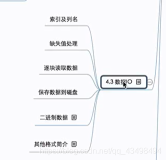
四、数据导入导出
数据IO,即可以从磁盘中读入数据,也可以将数据保存在磁盘上。例如:
通过网络爬虫,爬取一些数据过来,将数据通过解析以及清洗,最终保存类似.csv的文件,这个文件可能很大,pandas从文件中读出来,并对数据进行分析。pandas在读取文件会做许多操作。如下图:

说明:
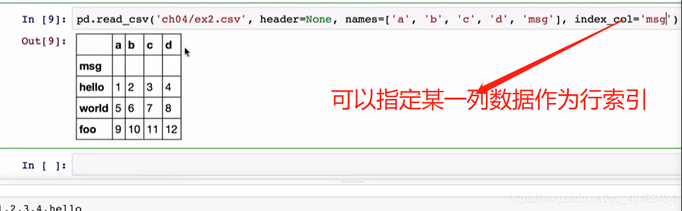
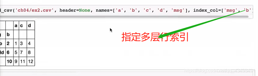
1索引可以自己指定或从文件中读取。
2如遇到整数就转换为整型,字符串就为字符串,以及浮点类型。
3遇到日期类型可以解析成Python中的日期类型,当然pandas也有自己的日期类型。
4pandas读取文件数据时,若文件数据很大,可以采取迭代读取一块,结合Python的迭代器或生成器算法来实现对大文件处理。
1

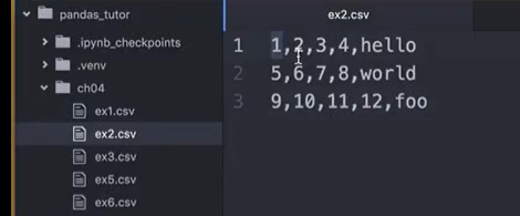
2读取文件数据,发现将文件第一行内容为列索引,行索引由pandas自动分配。

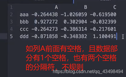
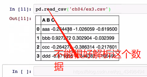
3对于一个文件若没有列名称,如下图:


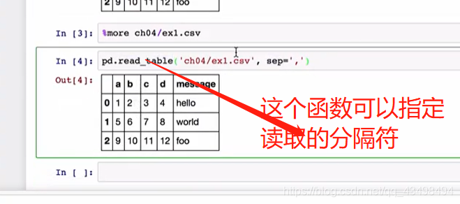
4看行索引
5处理不规则分隔符的文件数据的读取
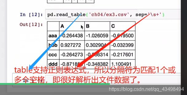

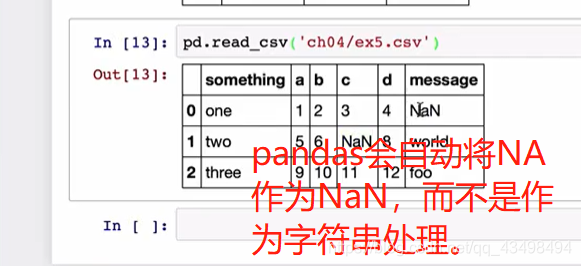
6对于文件数据中有缺失值的处理


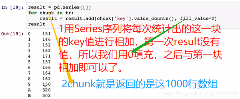
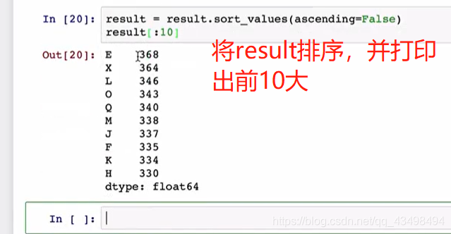
7逐块处理数据
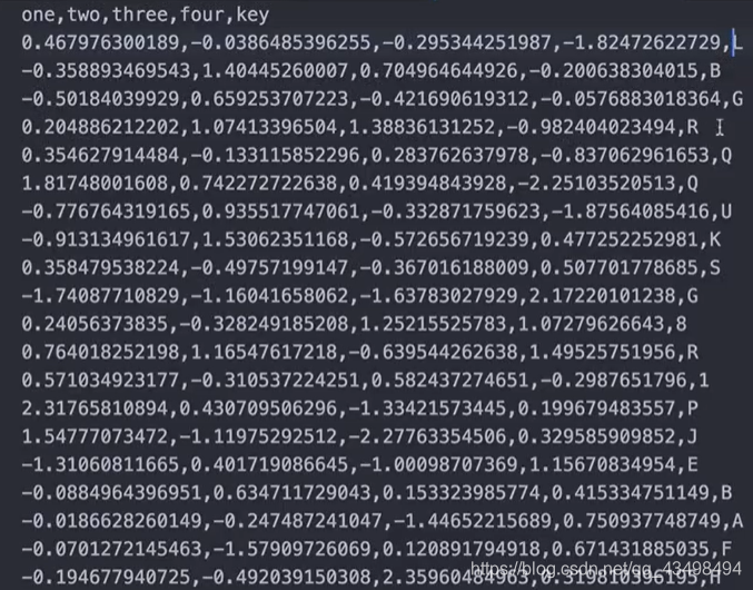
统计key对应下的各字母出现次数统计,并排序后打印出前10大,传统做法就是通过pandas将数据全部读出,用value_count统计即可,但是当文件几个G大小时,不可能一次读出来,所以要用分块统计,最后将和加起来。
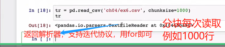
分块后每次用for循环迭代出时,都是1000行数据。
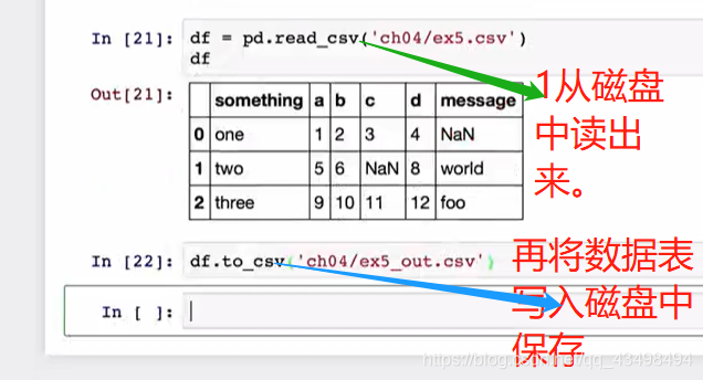
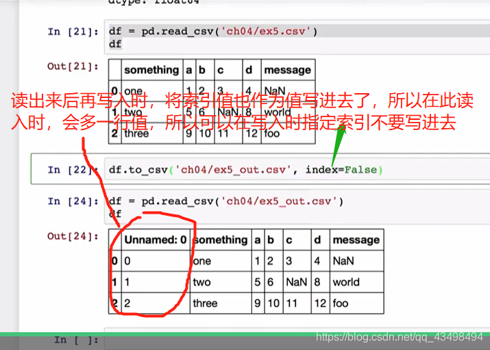
8将数据保存到磁盘中


二进制文件读取
容量小,读取速度块,因为二进制文件不需要解析。二进制数据实际上用python中饿pickle包来实现的。由于pickle包与pandas都会升级,所以早期保存的二进制数据再读回来时可能无法读出来。

其他格式简介

五、时间日期序列


datatime模块
rom datetime import datetime #导入时间函数
from datetime import timedelta  #导入时间之间的间隔
#1获取现在的时间
now=datetime.now()
print(now)
#2年月日
print(now.year,now.month, now.day)
#3创建2个时间,求出间隔timedelta 4 days
da1=datetime(2016,4,20)
da2=datetime(2016,4,16)
delta=da1-da2
#4取差的天数与秒数
print(delta.days)
print(delta.total_seconds())
#5
print(delta+da2)
#5加4.5天
print(da2+timedelta(4.5))
#6
da3=datetime(2016,3,20,8,30)
print(str(da3))#转成这种格式了。
#7strftime接受格式化的样式,将da3格式化,%Y大写4位年份,小写两位年份
da4=da3.strftime("%Y/%m/%d %H:%M:%S")
print(da4)
#8将一个字符串日期按照格式转化为datetime类型日期了
da5=datetime.strptime('2016-03-20 08:30',"%Y-%m-%d %H:%M")
print(da5)
print(type(da5))#<class 'datetime.datetime'>
结果:
D:\ProgramData\Anaconda3\python.exe D:/numpy-kexue/03.py
2020-01-15 10:31:44.393842
2020 1 15
4
345600.0
2016-04-20 00:00:00
2016-04-20 12:00:00
2016-03-20 08:30:00
2016/03/20 08:30:00
2016-03-20 08:30:00
<class 'datetime.datetime'>

Process finished with exit code 0
pandas中的时间日期序列
Timestamp时间戳即具体时间点信息
from datetime import datetime #导入时间函数
from datetime import timedelta #导入时间之间的间隔
#1用datetime创建一个序列作为索引出来
dates=[datetime(2016,3,1),datetime(2016,3,2),datetime(2016,3,3),datetime(2016,3,4)]
#2创建一个时间序列
s=pd.Series(np.random.randn(4),index=dates)
print(s)
print(type(s.index))#<class 'pandas.core.indexes.datetimes.DatetimeIndex'>
#DatetimeIndex是pandas中表示日期索引的结构。
print(type(s.index[0]))#pandas将datetime类型转化为Timestamp类型数据,来保存
#3pandas有自己生成时间序列的简单方法
#3生成时间戳序列的方法
s1=pd.date_range('20160320','20160330')
print(s1)#生成了一个DatetimeIndex的时间序列了, freq='D'周期默认以天为单位
#4用开始时间与个数如10个生成时间戳序列
s2=pd.date_range('20160320',periods=10)
print(s2)
#5生成带时刻的序列
s4=pd.date_range('20160320 16:32:38',periods=10)
print(s4)
#5去掉序列中的时分秒
s3=pd.date_range('20160320 16:32:38',periods=10,normalize=True)
print(s3)
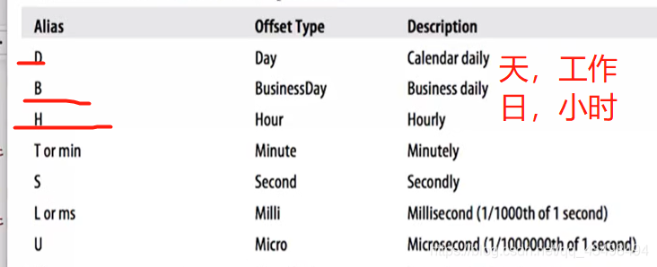
#6生成以天为频率的10个时间序列,频率可以指定为:W星期,M月份,以及BM每个月的最后一个工作日
#4H以4小时为频率
s5=pd.date_range('20160320',periods=10,freq='4H')
print(s5)
结果:
D:\ProgramData\Anaconda3\python.exe D:/numpy-kexue/03.py
2016-03-01 0.298983
2016-03-02 1.104373
2016-03-03 0.568569
2016-03-04 0.724501
dtype: float64
<class 'pandas.core.indexes.datetimes.DatetimeIndex'>
<class 'pandas._libs.tslibs.timestamps.Timestamp'>
DatetimeIndex(['2016-03-20', '2016-03-21', '2016-03-22', '2016-03-23',
'2016-03-24', '2016-03-25', '2016-03-26', '2016-03-27',
'2016-03-28', '2016-03-29', '2016-03-30'],
dtype='datetime64[ns]', freq='D')
DatetimeIndex(['2016-03-20', '2016-03-21', '2016-03-22', '2016-03-23',
'2016-03-24', '2016-03-25', '2016-03-26', '2016-03-27',
'2016-03-28', '2016-03-29'],
dtype='datetime64[ns]', freq='D')
DatetimeIndex(['2016-03-20 16:32:38', '2016-03-21 16:32:38',
'2016-03-22 16:32:38', '2016-03-23 16:32:38',
'2016-03-24 16:32:38', '2016-03-25 16:32:38',
'2016-03-26 16:32:38', '2016-03-27 16:32:38',
'2016-03-28 16:32:38', '2016-03-29 16:32:38'],
dtype='datetime64[ns]', freq='D')
DatetimeIndex(['2016-03-20', '2016-03-21', '2016-03-22', '2016-03-23',
'2016-03-24', '2016-03-25', '2016-03-26', '2016-03-27',
'2016-03-28', '2016-03-29'],
dtype='datetime64[ns]', freq='D')
DatetimeIndex(['2016-03-20 00:00:00', '2016-03-20 04:00:00',
'2016-03-20 08:00:00', '2016-03-20 12:00:00',
'2016-03-20 16:00:00', '2016-03-20 20:00:00',
'2016-03-21 00:00:00', '2016-03-21 04:00:00',
'2016-03-21 08:00:00', '2016-03-21 12:00:00'],
dtype='datetime64[ns]', freq='4H')
Process finished with exit code 0
pandas中的时期,时期不同于时间戳表示具体时间点,而是表示一个范围,如一年用电量,即一个时间范围。以下图片是在ipython notebook运行结果
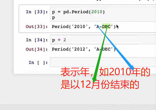
格式’A-DEC’列表:


#1创建一个表示2012年的时期
a=pd.Period(2012)
print(a)
#2做运算,就是2014了
print(a+2)
#3指定时期频率
b=pd.Period(2012,freq='M')
print(b)
print(b+2)
#4创建时期序列
c=pd.period_range('2016-01',periods=10,freq='M')
print(c)
#5创建时期序列PeriodIndex,并指定结束日期
c1=pd.period_range('2016-01','2016-12',freq='M')
print(c1)
#6创建季度时期序列,Q-DEC表示季度是以12月份为一年结束的单位
c2=pd.period_range('2016Q1',periods=10,freq='Q')
print(c2)
#7 a=pd.Period(2012) print(a)以年为单位的日期,要转化为以月为单位
c4=a.asfreq('M')#将2012转化为2012-12月了。默认以2012这一年结束的日期作为新的频率的日期。
print(c4)
#7变为1月份,将2012按照起始时间转化即可
c5=a.asfreq('M',how='start')#将2012转化为2012-12月了。默认以2012这一年结束的日期作为新的频率的日期。
print(c5)
#8创建一个月为频率的日期,并转化为年
c6=pd.Period('2016-04',freq='M')
print(c6)
c7=c6.asfreq('A-DEC')#转化为以年为单位,并以12月份结束的年
print(c7)#2016
#8将c6转化为以年为单位,且每年结束时间为3月份
c8=c6.asfreq('A-MAR')#转化为以年为单位,并以3月份结束的年
print(c8)#结果就是2017年
#9以季度频率并以1月份结束的季度频率
c9=pd.Period('2016Q4',freq='Q-JAN')
print(c9)
#具体查看2016Q4到底是?在Q-JAN这个时间段下的表示的起始与结束时间,
# 在Q-JAN这个时间段下通过转化为月份看2016Q4的起始与结束时间
c10=c9.asfreq('M',how='start'),c9.asfreq('M',how='end')
print(c10)
#将c9转换为以工作日B为单位的时期,表示第二个工作日下午4点20分
# 即在Q-JAN这个时间段下表示该季度下的倒数第二个工作日的下午4点20分
print((c9.asfreq('B')-1).asfreq('T'))#倒数第二个工作日,所以转化为工作日后减去1,再转化为分钟最后加上4点20份
#2016-01-28 23:59再加上16*60+20就是2016-01-29 16:19了。
print((c9.asfreq('B')-1).asfreq('T')+16*60+20)#倒数第二个工作日,所以转化为工作日后减去1,再转化为分钟最后加上4点20份
结果:
D:\ProgramData\Anaconda3\python.exe D:/numpy-kexue/03.py
2012
2014
2012-01
2012-03
PeriodIndex(['2016-01', '2016-02', '2016-03', '2016-04', '2016-05', '2016-06',
             '2016-07', '2016-08', '2016-09', '2016-10'],
            dtype='period[M]', freq='M')
PeriodIndex(['2016-01', '2016-02', '2016-03', '2016-04', '2016-05', '2016-06',
             '2016-07', '2016-08', '2016-09', '2016-10', '2016-11', '2016-12'],
            dtype='period[M]', freq='M')
PeriodIndex(['2016Q1', '2016Q2', '2016Q3', '2016Q4', '2017Q1', '2017Q2',
             '2017Q3', '2017Q4', '2018Q1', '2018Q2'],
            dtype='period[Q-DEC]', freq='Q-DEC')
2012-12
2012-01
2016-04
2016
2017
2016Q4
(Period('2015-11', 'M'), Period('2016-01', 'M'))
2016-01-28 23:59
2016-01-29 16:19

Process finished with exit code 0
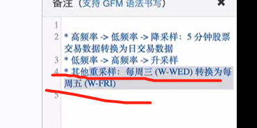
六、时间重采样

重采样:如股票交易数据是5分钟的频率改成日交易量,即高频率到低频率为降采样,还有低频率到高频率为升采样。
Timestamp与Period相互转化
注:Timestamp时间戳即具体时间点信息,pandas中的时期,时期Period
pd.period_range创建时期序列,pd.date_range创建时间戳序列。
mport  numpy as np
import  pandas as pd
s=pd.Series(np.random.randn(5),index=pd.date_range('2014-04-01',periods=5,freq='M'))
print(s)
#1将时间戳序列s转化为基于时期的序列
print(s.to_period())
#2以天为单位的序列,也转化为时期序列
s1=pd.Series(np.random.randn(5),index=pd.date_range('2016-12-29',periods=5,freq='D'))
print(s1)
print(s1.to_period())#转化为时期就是也是以天为频度了。
print(s1.to_period(freq='M'))#改为以月的频度
s2=s1.to_period(freq='M')
print(s2.index)#索引中有重复索引
s3=s2.groupby(level=0).sum()#level=0默认表示第1层行标签
print(s3)
#再将s2转化回为时间戳序列
print(s2)
s4=s2.to_timestamp()#可以看到将三个2016-12 月都转化为2016-12-01 了。
print(s4)
#转化为时间戳变为终止时间2016-12-31
s5=s2.to_timestamp(how='end')
print(s5)


#总之,从最初s1的2016-12-29 时间戳  转化为以月频度的时期s2变为2016-12 月,再转化为时间戳就变为2016-12-01 了。


结果:
D:\ProgramData\Anaconda3\python.exe D:/numpy-kexue/03.py
2014-04-30    0.726199
2014-05-31    0.022127
2014-06-30    0.426865
2014-07-31   -1.906621
2014-08-31    1.266856
Freq: M, dtype: float64
2014-04    0.726199
2014-05    0.022127
2014-06    0.426865
2014-07   -1.906621
2014-08    1.266856
Freq: M, dtype: float64
2016-12-29   -0.628399
2016-12-30    1.861908
2016-12-31   -0.654939
2017-01-01    0.453788
2017-01-02   -2.113595
Freq: D, dtype: float64
2016-12-29   -0.628399
2016-12-30    1.861908
2016-12-31   -0.654939
2017-01-01    0.453788
2017-01-02   -2.113595
Freq: D, dtype: float64
2016-12   -0.628399
2016-12    1.861908
2016-12   -0.654939
2017-01    0.453788
2017-01   -2.113595
Freq: M, dtype: float64
PeriodIndex(['2016-12', '2016-12', '2016-12', '2017-01', '2017-01'], dtype='period[M]', freq='M')
2016-12    0.578570
2017-01   -1.659807
Freq: M, dtype: float64
2016-12   -0.628399
2016-12    1.861908
2016-12   -0.654939
2017-01    0.453788
2017-01   -2.113595
Freq: M, dtype: float64
2016-12-01   -0.628399
2016-12-01    1.861908
2016-12-01   -0.654939
2017-01-01    0.453788
2017-01-01   -2.113595
dtype: float64
2016-12-31 23:59:59.999999999   -0.628399
2016-12-31 23:59:59.999999999    1.861908
2016-12-31 23:59:59.999999999   -0.654939
2017-01-31 23:59:59.999999999    0.453788
2017-01-31 23:59:59.999999999   -2.113595
dtype: float64

Process finished with exit code 0
重采样
import  numpy as np
import  pandas as pd

#1序列以时间戳分钟频度为索引,60个随机数,假设为某个股票一分钟成交量
s1=pd.Series(np.random.randint(0,50,60),index=pd.date_range('2016-4-25 09:30',periods=60,freq='T'))
print(s1)
#2将采样时间改为5min,聚合方式求和
s2=s1.resample('5min',how='sum')
#2016-04-25 09:30:00-2016-04-25 09:34:59这5分钟区间是以起始09:30:00为索引
print(s2)
#3若以每个区间的结束时间为索引,即2016-04-25 09:30:00-2016-04-25 09:34:59这5分钟区间是以起始09:34:59即记为9:35:00为索引,
# 只不过实际上数值累加是加到2016-04-25 09:34:59的只不过记为9:35:00了
s3=s1.resample('5min',how='sum',label='right')
print(s3)
#4将数据s1作为价格,即将每5分钟作为一个采样,有最高价格h,最低价格low,open开盘即起始价格,以及收盘价格cross
#求出每5分钟的价格,ohlc,开盘,最高,最低价,收盘价就可以方便求出来了。
s4=s1.resample('5min',how='ohlc')
print(s4)
结果:
D:\ProgramData\Anaconda3\python.exe D:/numpy-kexue/03.py
2016-04-25 09:30:00     7
2016-04-25 09:31:00     9
2016-04-25 09:32:00    28
2016-04-25 09:33:00    31
2016-04-25 09:34:00    11
2016-04-25 09:35:00     4
2016-04-25 09:36:00    10
2016-04-25 09:37:00    48
2016-04-25 09:38:00    15
2016-04-25 09:39:00    28
2016-04-25 09:40:00     6
2016-04-25 09:41:00    13
2016-04-25 09:42:00    49
2016-04-25 09:43:00    20
2016-04-25 09:44:00     6
2016-04-25 09:45:00    11
2016-04-25 09:46:00    42
2016-04-25 09:47:00    18
2016-04-25 09:48:00     8
2016-04-25 09:49:00     2
2016-04-25 09:50:00    47
2016-04-25 09:51:00    31
2016-04-25 09:52:00    35
2016-04-25 09:53:00    25
2016-04-25 09:54:00    42
2016-04-25 09:55:00    32
2016-04-25 09:56:00     2
2016-04-25 09:57:00    12
2016-04-25 09:58:00    31
2016-04-25 09:59:00    49
2016-04-25 10:00:00    33
2016-04-25 10:01:00    36
2016-04-25 10:02:00    38
2016-04-25 10:03:00    45
2016-04-25 10:04:00    17
2016-04-25 10:05:00    28
2016-04-25 10:06:00    10
2016-04-25 10:07:00    10
2016-04-25 10:08:00    32
2016-04-25 10:09:00    45
2016-04-25 10:10:00    10
2016-04-25 10:11:00    29
2016-04-25 10:12:00     7
2016-04-25 10:13:00    36
2016-04-25 10:14:00     0
2016-04-25 10:15:00    18
2016-04-25 10:16:00    24
2016-04-25 10:17:00    49
2016-04-25 10:18:00    46
2016-04-25 10:19:00    29
2016-04-25 10:20:00    46
2016-04-25 10:21:00    37
2016-04-25 10:22:00    42
2016-04-25 10:23:00    33
2016-04-25 10:24:00    36
2016-04-25 10:25:00    11
2016-04-25 10:26:00     2
2016-04-25 10:27:00    22
2016-04-25 10:28:00    39
2016-04-25 10:29:00    32
Freq: T, dtype: int32
D:/numpy-kexue/03.py:563: FutureWarning: how in .resample() is deprecated
the new syntax is .resample(...).sum()
  s2=s1.resample('5min',how='sum')
D:/numpy-kexue/03.py:568: FutureWarning: how in .resample() is deprecated
the new syntax is .resample(...).sum()
  s3=s1.resample('5min',how='sum',label='right')
D:/numpy-kexue/03.py:572: FutureWarning: how in .resample() is deprecated
the new syntax is .resample(...).ohlc()
  s4=s1.resample('5min',how='ohlc')
2016-04-25 09:30:00     86
2016-04-25 09:35:00    105
2016-04-25 09:40:00     94
2016-04-25 09:45:00     81
2016-04-25 09:50:00    180
2016-04-25 09:55:00    126
2016-04-25 10:00:00    169
2016-04-25 10:05:00    125
2016-04-25 10:10:00     82
2016-04-25 10:15:00    166
2016-04-25 10:20:00    194
2016-04-25 10:25:00    106
Freq: 5T, dtype: int32
2016-04-25 09:35:00     86
2016-04-25 09:40:00    105
2016-04-25 09:45:00     94
2016-04-25 09:50:00     81
2016-04-25 09:55:00    180
2016-04-25 10:00:00    126
2016-04-25 10:05:00    169
2016-04-25 10:10:00    125
2016-04-25 10:15:00     82
2016-04-25 10:20:00    166
2016-04-25 10:25:00    194
2016-04-25 10:30:00    106
Freq: 5T, dtype: int32
                     open  high  low  close
2016-04-25 09:30:00     7    31    7     11
2016-04-25 09:35:00     4    48    4     28
2016-04-25 09:40:00     6    49    6      6
2016-04-25 09:45:00    11    42    2      2
2016-04-25 09:50:00    47    47   25     42
2016-04-25 09:55:00    32    49    2     49
2016-04-25 10:00:00    33    45   17     17
2016-04-25 10:05:00    28    45   10     45
2016-04-25 10:10:00    10    36    0      0
2016-04-25 10:15:00    18    49   18     29
2016-04-25 10:20:00    46    46   33     36
2016-04-25 10:25:00    11    39    2     32

Process finished with exit code 0
import  numpy as np
import  pandas as pd

#1通过groupby重采样,100天为单位频度
s1=pd.Series(np.random.randint(0,50,100),index=pd.date_range('2016-3-01 09:30',periods=100,freq='D'))
print(s1)
#2基于月份x.month重采样,x是s1的索引日期值,将3月份所有数据都加起来了,以及4月份数据所有加起来
s2=s1.groupby(lambda  x:x.month).sum()
print(s2)
#2 s1.index就是时间戳序列转化为时期序列,以月为频度,之后就是按照月份分组了
s3=s1.groupby(s1.index.to_period('M')).sum()
print(s3)#与s2一样只不过前边索引表示不一样
print(type(s3.index))#PeriodIndex就是时期序列了。
结果:
D:\ProgramData\Anaconda3\python.exe D:/numpy-kexue/03.py
2016-03-01 09:30:00    22
2016-03-02 09:30:00    15
2016-03-03 09:30:00     8
2016-03-04 09:30:00     9
2016-03-05 09:30:00     0
2016-03-06 09:30:00     1
2016-03-07 09:30:00    33
2016-03-08 09:30:00    21
2016-03-09 09:30:00    47
2016-03-10 09:30:00    22
2016-03-11 09:30:00    35
2016-03-12 09:30:00    43
2016-03-13 09:30:00    13
2016-03-14 09:30:00    29
2016-03-15 09:30:00    44
2016-03-16 09:30:00    25
2016-03-17 09:30:00    25
2016-03-18 09:30:00    49
2016-03-19 09:30:00     5
2016-03-20 09:30:00    43
2016-03-21 09:30:00     2
2016-03-22 09:30:00    27
2016-03-23 09:30:00    35
2016-03-24 09:30:00    43
2016-03-25 09:30:00    28
2016-03-26 09:30:00    16
2016-03-27 09:30:00    17
2016-03-28 09:30:00    30
2016-03-29 09:30:00    29
2016-03-30 09:30:00    31
                       ..
2016-05-10 09:30:00     8
2016-05-11 09:30:00    27
2016-05-12 09:30:00     4
2016-05-13 09:30:00    36
2016-05-14 09:30:00    31
2016-05-15 09:30:00    16
2016-05-16 09:30:00    43
2016-05-17 09:30:00    28
2016-05-18 09:30:00    48
2016-05-19 09:30:00    46
2016-05-20 09:30:00     3
2016-05-21 09:30:00    42
2016-05-22 09:30:00    42
2016-05-23 09:30:00    22
2016-05-24 09:30:00    15
2016-05-25 09:30:00     4
2016-05-26 09:30:00    24
2016-05-27 09:30:00    26
2016-05-28 09:30:00    46
2016-05-29 09:30:00    42
2016-05-30 09:30:00    47
2016-05-31 09:30:00    38
2016-06-01 09:30:00    47
2016-06-02 09:30:00    27
2016-06-03 09:30:00    16
2016-06-04 09:30:00    42
2016-06-05 09:30:00    23
2016-06-06 09:30:00    20
2016-06-07 09:30:00    21
2016-06-08 09:30:00    35
Freq: D, Length: 100, dtype: int32
3    758
4    613
5    851
6    231
dtype: int32
2016-03    758
2016-04    613
2016-05    851
2016-06    231
Freq: M, dtype: int32
<class 'pandas.core.indexes.period.PeriodIndex'>

Process finished with exit code 0
升采样
import  numpy as np
import  pandas as pd

#1时间戳序列以周为单位,结束为周五的频度,即每周五为每周的结束
s1=pd.DataFrame(np.random.randint(1,50,2),index=pd.date_range('2016-04-22 ',periods=2,freq='W-FRI'))
print(s1)
#2以周为单位数据转化为以天为单位的数据,涉及插值了,因为4-22到4-29本来没有值,
# 所以现在以天为单位就要有值,所以要插值
#2插值默认时填NaN进去
s2=s1.resample('D')
print(s2)
#3插值ffill就是后面的数字默认都是向前面插值
s3=s1.resample('D',fill_method='ffill')
print(s3)
#4设置期限,即最多向前面数字插值插3个,离前面的数字超过3个的NaN即还是NaN了。。
s4=s1.resample('D',fill_method='ffill',limit=3)
print(s4)
#5W-FRI'转化为以'W-MON以周为单位且周一结束的单位的频度
s5=s1.resample('W-MON',fill_method='ffill')
print(s5)#4-22 是周五,下周的周一就是4-25了
结果:
D:\ProgramData\Anaconda3\python.exe D:/numpy-kexue/03.py
             0
2016-04-22  10
2016-04-29   5
DatetimeIndexResampler [freq=<Day>, axis=0, closed=left, label=left, convention=start, base=0]
D:/numpy-kexue/03.py:568: FutureWarning: fill_method is deprecated to .resample()
the new syntax is .resample(...).ffill()
  s3=s1.resample('D',fill_method='ffill')
D:/numpy-kexue/03.py:571: FutureWarning: fill_method is deprecated to .resample()
the new syntax is .resample(...).ffill(limit=3)
  s4=s1.resample('D',fill_method='ffill',limit=3)
D:/numpy-kexue/03.py:574: FutureWarning: fill_method is deprecated to .resample()
the new syntax is .resample(...).ffill()
  s5=s1.resample('W-MON',fill_method='ffill')
             0
2016-04-22  10
2016-04-23  10
2016-04-24  10
2016-04-25  10
2016-04-26  10
2016-04-27  10
2016-04-28  10
2016-04-29   5
               0
2016-04-22  10.0
2016-04-23  10.0
2016-04-24  10.0
2016-04-25  10.0
2016-04-26   NaN
2016-04-27   NaN
2016-04-28   NaN
2016-04-29   5.0
             0
2016-04-25  10
2016-05-02   5

Process finished with exit code 0
#1时期序列以月为单位
s1=pd.DataFrame(np.random.randint(2,30,(24,4)),index=pd.period_range('2015-01','2016-12 ',freq='M'),columns=list('ABCD'))
print(s1)
# 2重采样为以年为单位的且以12月份结束的
s2=s1.resample('A-DEC',how='mean')#默认求平均值
print(s2)
s3=s1.resample('A-DEC',how='sum')#默认求平均值
print(s3)
#以年为单位的且以3月份结束的,#此时有三个年份了,2015是2015-01 到2015-03累加值,
#2016是2015-04 到2016-03累加值,最后是2017累加值了。
s4=s1.resample('A-MAR',how='sum')#默认求平均值
print(s4)
结果:
D:\ProgramData\Anaconda3\python.exe D:/numpy-kexue/03.py
          A   B   C   D
D:/numpy-kexue/03.py:563: FutureWarning: how in .resample() is deprecated
2015-01  15   8  21  11
the new syntax is .resample(...).mean()
2015-02  26   2  26  10
  s2=s1.resample('A-DEC',how='mean')#默认求平均值
2015-03   8  24  23   3
2015-04  12  28  20  16
2015-05  28  13  23   5
2015-06   6  10  19  13
2015-07   8  15   5  11
2015-08  10  12   6  16
2015-09  24   8  14  24
2015-10  17  11   8   3
2015-11  28   6  27  29
2015-12  15   4  11  20
2016-01  22   3  22   5
2016-02  14   6  18  21
2016-03   3  25  28   9
2016-04  15  17  29   8
2016-05  28  22   2   6
2016-06   8  18  17  22
2016-07  24  24   4   2
2016-08  29   6   2   5
2016-09  19  19  22   3
2016-10  16  14  13  21
2016-11   3  14  14   8
2016-12  29   6  28  15
              A      B          C          D
2015  16.416667  11.75  16.916667  13.416667
2016  17.500000  14.50  16.583333  10.416667
D:/numpy-kexue/03.py:565: FutureWarning: how in .resample() is deprecated
the new syntax is .resample(...).sum()
  s3=s1.resample('A-DEC',how='sum')#默认求平均值
        A    B    C    D
2015  197  141  203  161
2016  210  174  199  125
        A    B    C    D
2015   49   34   70   24
2016  187  141  201  172
2017  171  140  131   90
D:/numpy-kexue/03.py:568: FutureWarning: how in .resample() is deprecated
the new syntax is .resample(...).sum()
  s4=s1.resample('A-MAR',how='sum')#默认求平均值

Process finished with exit code 0
import  numpy as np
import  pandas as pd

#1时期序列以月为单位
s1=pd.DataFrame(np.random.randint(2,30,(24,4)),index=pd.period_range('2015-01','2016-12 ',freq='M'),columns=list('ABCD'))
print(s1)
# 2两年的数据
s2=s1.resample('A-DEC',how='mean')#默认求平均值
print(s2)
#3以季度采样,并未指定填充方法,所以都是NaN
s3=s2.resample('Q-DEC')
print(s3)
#3以季度采样,向前填充
s4=s2.resample('Q-DEC',fill_method='ffill')
print(s4)
结果:
D:\ProgramData\Anaconda3\python.exe D:/numpy-kexue/03.py
          A   B   C   D
2015-01  18   2   2   9
2015-02  13  15  27  12
2015-03  29   6  10  16
2015-04   6  16  10   4
2015-05  15  17  11  18
2015-06  23  17  28  26
2015-07  26  18  10  28
2015-08  28   9  28  27
2015-09  22  25  19  20
2015-10  28   3  13  22
2015-11  26   2  12  20
2015-12  28   5  10  25
2016-01   7   9  11   4
2016-02   9  14  18  29
2016-03  13  23   7  23
2016-04  28   7   2  24
2016-05  26  20  22   3
2016-06  25  17  22  21
2016-07  23  27   7   6
2016-08  11  23   2  13
2016-09  23  17  21   6
2016-10  16  13  28  29
2016-11  10   5  15  19
2016-12  19  14  11   7
D:/numpy-kexue/03.py:563: FutureWarning: how in .resample() is deprecated
the new syntax is .resample(...).mean()
  s2=s1.resample('A-DEC',how='mean')#默认求平均值
              A      B          C          D
D:/numpy-kexue/03.py:569: FutureWarning: fill_method is deprecated to .resample()
the new syntax is .resample(...).ffill()
  s4=s2.resample('Q-DEC',fill_method='ffill')
2015  21.833333  11.25  15.000000  18.916667
2016  17.500000  15.75  13.833333  15.333333
PeriodIndexResampler [freq=<QuarterEnd: startingMonth=12>, axis=0, closed=right, label=right, convention=start, base=0]
                A      B          C          D
2015Q1  21.833333  11.25  15.000000  18.916667
2015Q2  21.833333  11.25  15.000000  18.916667
2015Q3  21.833333  11.25  15.000000  18.916667
2015Q4  21.833333  11.25  15.000000  18.916667
2016Q1  17.500000  15.75  13.833333  15.333333
2016Q2  17.500000  15.75  13.833333  15.333333
2016Q3  17.500000  15.75  13.833333  15.333333
2016Q4  17.500000  15.75  13.833333  15.333333

Process finished with exit code 0

从文件中解析出时间序列


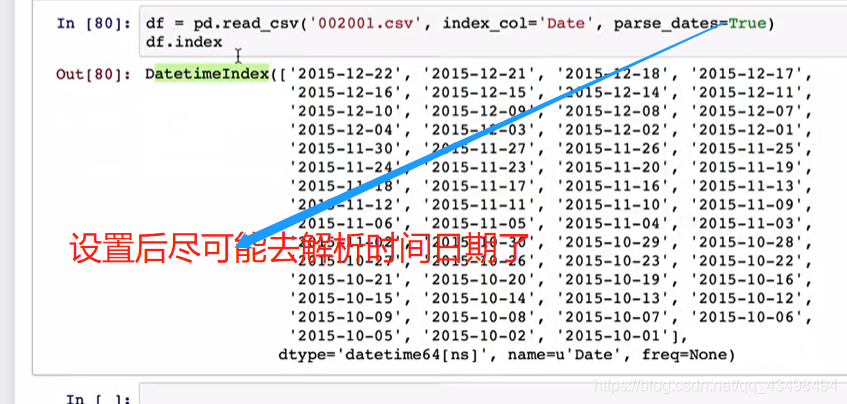
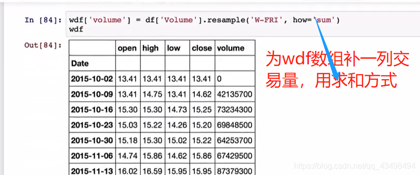
时间日期解析后就可以重采样了。将日交易数据转化为周交易数据了。如下图


可以看到每周的交易量了。
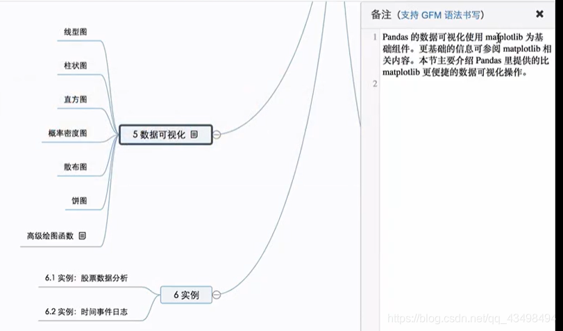
六、数据可视化

一维数组线形图
通过线形图来观察一些数据变化规律。
import numpy as np
import pandas as pd
import matplotlib.pyplot as plt
#1创建1000个点
s=pd.Series(np.random.randn(1000),index=pd.date_range('2000/1/1',periods=1000))
print(s)
#2累积求和
s1=s.cumsum()
print(s1)
print(s1.describe())
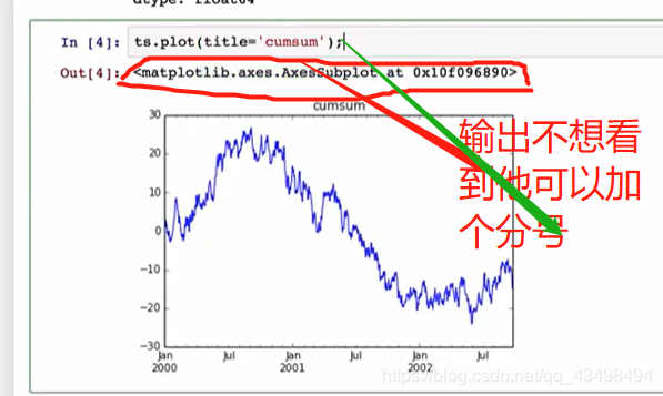
#3画图线形图,默认是实线,加个标签,颜色红色以及虚线,设置图片大小,单位英寸
print(s1.plot(title='consum',style='r--',figsize=(8,6)))
#显示在pycharm中,有图像了。即在幕布上显示
plt.show()
结果:
D:\ProgramData\Anaconda3\python.exe D:/numpy-kexue/03.py
2000-01-01 0.021750
2000-01-02 -0.342224
2000-01-03 -0.703360
2000-01-04 -0.080740
2000-01-05 0.839622
2000-01-06 -0.623088
2000-01-07 1.250108
2000-01-08 -2.248451
2000-01-09 -0.071523
2000-01-10 -0.453560
2000-01-11 0.230066
2000-01-12 0.200287
2000-01-13 1.278155
2000-01-14 -0.101347
2000-01-15 0.943621
2000-01-16 1.541332
2000-01-17 0.355654
2000-01-18 -0.604720
2000-01-19 -1.850330
2000-01-20 -1.096652
2000-01-21 -0.484040
2000-01-22 0.814972
2000-01-23 -0.586763
2000-01-24 0.139452
2000-01-25 -0.406494
2000-01-26 -0.093064
2000-01-27 0.643097
2000-01-28 -0.089406
2000-01-29 -0.545005
2000-01-30 1.563478
...
2002-08-28 0.040647
2002-08-29 -0.123445
2002-08-30 -1.523656
2002-08-31 -1.033728
2002-09-01 -1.070606
2002-09-02 0.157957
2002-09-03 -1.748463
2002-09-04 1.274990
2002-09-05 0.687259
2002-09-06 0.260984
2002-09-07 0.626288
2002-09-08 0.369706
2002-09-09 -0.139057
2002-09-10 0.328967
2002-09-11 0.451696
2002-09-12 0.062908
2002-09-13 -1.480679
2002-09-14 -1.022592
2002-09-15 -0.767008
2002-09-16 -0.188620
2002-09-17 -0.223606
2002-09-18 1.040383
2002-09-19 0.961064
2002-09-20 -0.367202
2002-09-21 0.521306
2002-09-22 0.221847
2002-09-23 -0.358859
2002-09-24 0.908444
2002-09-25 -1.371190
2002-09-26 0.903915
Freq: D, Length: 1000, dtype: float64
2000-01-01 0.021750
2000-01-02 -0.320474
2000-01-03 -1.023834
2000-01-04 -1.104574
2000-01-05 -0.264952
2000-01-06 -0.888040
2000-01-07 0.362068
2000-01-08 -1.886383
2000-01-09 -1.957906
2000-01-10 -2.411466
2000-01-11 -2.181400
2000-01-12 -1.981113
2000-01-13 -0.702957
2000-01-14 -0.804305
2000-01-15 0.139317
2000-01-16 1.680649
2000-01-17 2.036303
2000-01-18 1.431583
2000-01-19 -0.418747
2000-01-20 -1.515399
2000-01-21 -1.999439
2000-01-22 -1.184467
2000-01-23 -1.771230
2000-01-24 -1.631778
2000-01-25 -2.038273
2000-01-26 -2.131337
2000-01-27 -1.488239
2000-01-28 -1.577645
2000-01-29 -2.122650
2000-01-30 -0.559172
...
2002-08-28 -13.562599
2002-08-29 -13.686044
2002-08-30 -15.209699
2002-08-31 -16.243428
2002-09-01 -17.314034
2002-09-02 -17.156078
2002-09-03 -18.904540
2002-09-04 -17.629550
2002-09-05 -16.942291
2002-09-06 -16.681308
2002-09-07 -16.055020
2002-09-08 -15.685314
2002-09-09 -15.824371
2002-09-10 -15.495405
2002-09-11 -15.043708
2002-09-12 -14.980800
2002-09-13 -16.461479
2002-09-14 -17.484072
2002-09-15 -18.251080
2002-09-16 -18.439699
2002-09-17 -18.663305
2002-09-18 -17.622922
2002-09-19 -16.661859
2002-09-20 -17.029060
2002-09-21 -16.507754
2002-09-22 -16.285907
2002-09-23 -16.644765
2002-09-24 -15.736321
2002-09-25 -17.107512
2002-09-26 -16.203597
Freq: D, Length: 1000, dtype: float64
count 1000.000000
mean 4.458359
std 9.849305
min -18.904540
25% -3.129378
50% 6.714317
75% 11.469969
max 23.148331
dtype: float64
AxesSubplot(0.125,0.11;0.775x0.77)
Process finished with exit code 0
二维数组线形图
import  numpy as np
import  pandas as pd
import  matplotlib.pyplot as plt

#1创建1000个点
s=pd.Series(np.random.randn(1000),index=pd.date_range('2000/1/1',periods=1000))
s1=pd.DataFrame(np.random.randn(1000,4),  index=s.index,columns=list('ABCD'))
#1累积求和
s2=s1.cumsum()
print(s2)
print(s2.describe())
#2将x轴时间标签,y轴数值自动给我们弄好了,即pandas使用 matplotlib这个基础组件,
# 但是比 matplotlib这个基础组件使用起来更方便的可视化操作。如将x轴时间标签,y轴数值自动给我们弄好了
print(s2.plot())
#3二维数组除了画图线形图,默认是实线,加个标签,颜色红色以及虚线,设置图片大小,单位英寸特习性即
# title='consum',style='r--',figsize=(8,6)外,还有如将每个列标签单独画成子图显示即4个图
print(s2.plot(subplots=True,figsize=(6,12)))
#4默认x轴共用,y轴不同,可以让y轴变成一样,此时y轴都是-30-40了。
print(s2.plot(subplots=True,figsize=(6,12),sharey=True))
#5默认与Series一样将索引作为x轴,也可以指定。
#增加一列ID,指定ID为x轴
s2['ID']=np.arange(len(s1))
# print(s1)
s3=s1.describe()
print(s3)
print(s2.plot(x='ID',y=['A','C']))
#4显示在pycharm中,有图像了。即在幕布上显示
plt.show()
结果:
D:\ProgramData\Anaconda3\python.exe D:/numpy-kexue/03.py
                    A          B          C          D
2000-01-01   0.043858  -1.938042   0.066523   1.442944
2000-01-02   1.795494  -3.642003   0.555598   0.858347
2000-01-03  -0.359311  -3.820776  -0.432168   0.794428
2000-01-04   0.512016  -3.450523  -1.072690   0.041339
2000-01-05   1.496142  -2.645604  -0.820479   2.390145
2000-01-06   2.711531  -1.414371  -2.447141   1.533634
2000-01-07   3.243149  -2.580588  -2.928076   0.274428
2000-01-08   3.816423  -4.117339  -2.322788   0.823162
2000-01-09   5.355620  -3.497706  -4.303406   1.715052
2000-01-10   5.317233  -3.057616  -5.880139   1.438897
2000-01-11   4.882865  -2.114240  -6.940608   1.579358
2000-01-12   5.415567  -0.147245  -7.004251   1.530874
2000-01-13   4.432608  -0.037263  -9.772249   2.102540
2000-01-14   4.391335   1.293968 -11.177027   1.896847
2000-01-15   3.728721   1.002861 -11.350167   2.680543
2000-01-16   3.303002  -1.921472 -11.310425   4.427158
2000-01-17   2.675820  -2.621257 -10.425633   4.721797
2000-01-18   3.289668  -1.642567  -9.510580   6.370149
2000-01-19   3.342545  -2.218178  -7.802074   6.914362
2000-01-20   2.351196  -2.935037  -8.054005   7.071771
2000-01-21   1.055081  -1.736253  -8.510524   7.390703
2000-01-22   1.486078  -0.143644  -7.340185   6.502912
2000-01-23   1.533922  -0.011707  -7.127269   6.804994
2000-01-24   1.270045  -0.997774  -8.541212   5.982335
2000-01-25   1.980192   0.821598  -8.391792   8.227305
2000-01-26   3.054330   2.029531  -7.499317   9.927661
2000-01-27   1.701030   1.906175  -8.817998   8.723671
2000-01-28   1.712898   1.913258 -10.928263   7.539682
2000-01-29   2.987447   2.491506 -11.899118   6.853198
2000-01-30   2.724693   1.477739 -12.682139   7.393432
...               ...        ...        ...        ...
2002-08-28  35.904782 -16.741661 -13.343951 -48.029499
2002-08-29  35.855188 -17.230687 -13.111510 -47.411871
2002-08-30  37.427582 -17.914023 -13.666857 -46.829978
2002-08-31  37.731211 -17.597448 -13.504501 -48.355345
2002-09-01  36.265599 -18.403235 -12.482321 -48.442303
2002-09-02  36.733513 -18.332368 -12.507712 -48.395870
2002-09-03  37.369288 -19.714581 -11.450133 -49.787907
2002-09-04  38.718678 -20.314891 -12.197848 -49.707121
2002-09-05  37.898109 -18.916117 -11.952324 -48.138423
2002-09-06  37.995770 -17.734368 -13.131787 -47.647642
2002-09-07  36.387358 -17.324411 -11.934539 -48.324773
2002-09-08  37.079347 -16.898558 -12.175339 -48.097957
2002-09-09  36.330430 -15.578053 -11.538078 -45.651228
2002-09-10  36.795977 -16.825679 -11.607556 -46.190043
2002-09-11  35.956330 -18.878719 -11.208667 -47.524849
2002-09-12  35.467328 -19.637815 -10.246662 -47.987226
2002-09-13  33.822880 -20.575757 -12.050516 -49.820369
2002-09-14  35.829691 -21.735511 -12.153652 -49.721350
2002-09-15  35.851353 -20.142455 -13.381996 -49.869945
2002-09-16  36.477656 -18.811438 -15.568471 -49.367486
2002-09-17  36.059301 -18.969181 -15.819040 -48.678801
2002-09-18  37.320086 -19.230842 -17.503732 -48.837032
2002-09-19  36.236123 -20.594255 -17.434688 -47.903998
2002-09-20  35.166057 -20.382245 -18.176208 -47.838766
2002-09-21  33.455785 -21.385285 -18.248580 -47.663114
2002-09-22  33.477029 -21.443371 -18.295012 -46.977856
2002-09-23  33.803563 -22.061559 -17.893184 -46.744404
2002-09-24  31.473179 -22.613393 -18.473440 -45.290860
2002-09-25  32.617691 -21.239231 -17.692620 -44.504582
2002-09-26  34.232243 -22.129346 -19.572509 -45.672834

[1000 rows x 4 columns]
                 A            B            C            D
count  1000.000000  1000.000000  1000.000000  1000.000000
mean     20.402215     7.738370   -17.141770   -27.823476
std       7.817633    10.164835     8.450942    17.126514
min      -0.359311   -22.613393   -39.963882   -55.558537
25%      15.707210     3.946894   -22.641156   -39.900693
50%      20.250860     8.786266   -16.667624   -33.912291
75%      25.357199    14.768713   -10.698475   -15.373469
max      38.718678    25.012509     0.555598     9.927661
AxesSubplot(0.125,0.11;0.775x0.77)
                 A            B            C            D
count  1000.000000  1000.000000  1000.000000  1000.000000
mean      0.034232    -0.022129    -0.019573    -0.045673
std       0.997916     0.976747     0.968159     0.997014
min      -3.053475    -3.100115    -3.080448    -4.514357
25%      -0.669360    -0.693916    -0.679502    -0.716968
50%       0.061978    -0.046314    -0.045284    -0.040341
75%       0.691326     0.616256     0.635363     0.605444
max       3.389259     2.857237     3.279545     3.781553
AxesSubplot(0.125,0.11;0.775x0.77)

Process finished with exit code 0
柱状图
```python
import  numpy as np
import  pandas as pd
import  matplotlib.pyplot as plt


s1=pd.DataFrame(np.random.randn(10,4), columns=list('ABCD'))
print(s1)
#1针对画了第一行的柱状图
print(s1.iloc[0].plot(kind='bar'))
#2将所有柱状图画在一起,即每一个点就是对应ABCD 4列
print(s1.plot.bar())
#3将ABCD堆叠起来画柱状图
print(s1.plot.bar(stacked=True))
#4画水平方向柱状图
print(s1.plot.barh(stacked=True))
结果:
D:\ProgramData\Anaconda3\python.exe D:/numpy-kexue/03.py
          A         B         C         D
0 -1.170778 -1.117512 -0.223939 -0.098151
1  1.410190 -1.265715  1.088915 -0.170983
2 -0.632128  0.901031  0.815459 -0.029714
3  0.429248  0.637022 -0.269711  2.341861
4  2.174755 -1.156607 -0.438013 -1.842582
5  1.006937 -0.354087 -1.608195  0.446598
6 -0.127342 -0.839094  0.139954 -0.483935
7 -1.152274  0.689993 -0.300963  0.150271
8  2.325571  0.017893  1.185659 -0.777143
9 -0.571188 -0.777967  0.843428  0.551264
AxesSubplot(0.125,0.11;0.775x0.77)
AxesSubplot(0.125,0.11;0.775x0.77)
AxesSubplot(0.125,0.11;0.775x0.77)
AxesSubplot(0.125,0.11;0.775x0.77)

Process finished with exit code 0
直方图
import numpy as np
import pandas as pd
import matplotlib.pyplot as plt
df1=pd.DataFrame({'a':np.random.randn(1000)+1,
'b':np.random.randn(1000),
'c':np.random.randn(1000)-1},columns=['a','b','c'])
print(df1)
#1针对a这一列画的直方图bins=20,有20个柱子出来
# 即a这一列,将最小值与最大值分成20等分,每个区间的点的个数为y轴,x轴就是等分点
print(df1['a'].hist(bins=20))#可以发现在1附近点数就多,因为就是用正态分布产生的点,所以直方图也近似服从正态分布
#2将df1的4列都画出来,4个子图,且x轴坐标要一样共用sharex=True,y轴也一样共用sharey=True
print(df1.plot.hist(subplots=True,sharex=True,sharey=True))
#因为a是正态分布均值0+1所以a在1附近,同理b在0附近,c在-1附近。
#3df1.plot默认画的是线形图
#4将图放在一个图片里
print(df1.plot.hist())
#5透明度设置
print(df1.plot.hist(alpha=0.3))
#6画成叠加的看,数据集中在0附近,可以不透明,去掉alpha=0.3
print(df1.plot.hist(stacked=True))
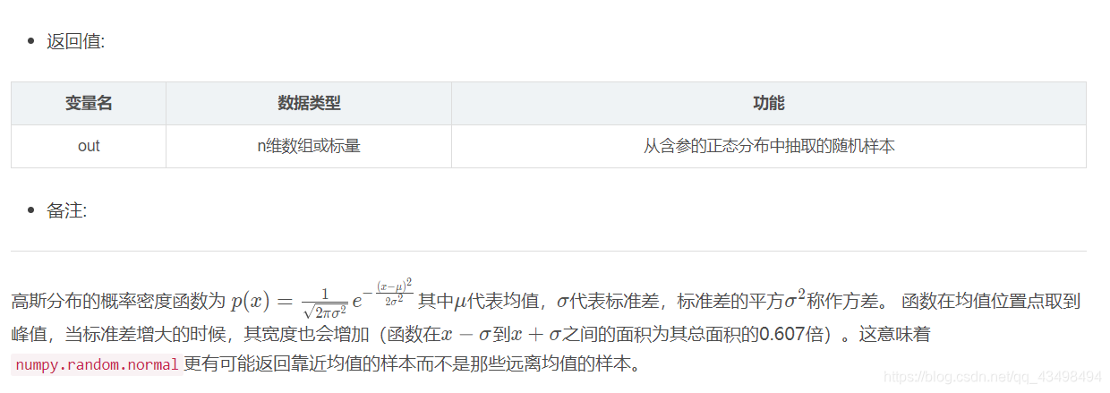
#7概率密度可以衡量一个事件发生概率的大小。
#画出a的概率密度函数,且近似是正态分布
print(df1['a'].plot.kde())
#画出所有标签概率密度函数,且近似是正态分布
print(df1.plot.kde())
#8因为正态分布由均值方差决定,均值决定概率密度中心点位置
print(df1.mean())
#9方差决定概率密度的宽窄
print(df1.std())#三个方差差不多大,所以形状类似。
plt.show()
结果:
D:\ProgramData\Anaconda3\python.exe D:/numpy-kexue/03.py
a b c
0 3.272862 -1.225387 -1.954024
1 1.024334 -0.130112 -0.207561
2 1.185716 0.355673 -0.554698
3 1.931817 -1.762353 -1.325085
4 1.418963 0.235359 -0.543921
5 0.821318 -0.399454 -0.762425
6 2.032535 0.671341 -1.327233
7 3.080431 -0.450417 -0.692577
8 0.666281 -1.077308 -0.971437
9 1.024319 -1.423796 -2.409847
10 2.140859 1.249195 -2.120990
11 0.822096 0.005720 -2.929745
12 1.373357 0.733599 -1.133428
13 0.671509 0.055096 -1.359616
14 1.488930 0.074107 -1.469906
15 2.721467 0.683869 -0.565490
16 1.765766 0.152811 -0.436782
17 0.863173 1.652283 -0.087714
18 1.311450 -1.190876 -0.601183
19 1.528339 0.097765 -0.366915
20 2.711436 0.661133 -0.988031
21 1.443029 -0.542094 -2.395894
22 -0.554260 -0.655259 -1.223408
23 0.589265 -0.304013 -1.045963
24 -0.293028 -0.808648 -0.987862
25 1.659238 -0.250684 -0.473819
26 1.055222 -0.659888 -0.256713
27 -0.074811 -0.725006 -0.965644
28 0.777949 0.155333 -1.084517
29 1.015265 -0.887539 -0.258392
.. ... ... ...
970 1.119371 0.340837 -0.393762
971 -2.065207 1.900022 -1.205609
972 2.327063 0.375810 -0.754037
973 1.607693 -0.151844 -0.318051
974 0.745030 0.568752 -1.177329
975 2.779861 0.895405 -2.665706
976 1.290887 0.554768 -1.061650
977 0.793900 -0.287829 0.874936
978 -0.746711 0.269235 -2.556524
979 2.092600 0.249613 -0.896967
980 1.899295 -0.181241 0.008159
981 0.028985 1.759899 -1.998670
982 1.401252 -1.849261 0.315134
983 -0.086929 0.677276 -1.314479
984 1.638782 0.574020 -0.624601
985 0.528698 0.620596 -1.153925
986 2.332607 -0.272598 0.526256
987 1.686126 0.737786 -1.517588
988 -0.495981 -1.386138 -1.492892
989 0.449099 -2.077898 -1.056452
990 0.705737 0.285780 -0.659085
991 1.648441 0.124969 -0.179757
992 1.268579 -1.114629 -0.265299
993 1.572413 -0.198383 -1.598407
994 1.103471 0.342782 0.466902
995 1.097359 -0.190465 -1.521666
996 1.215999 0.434159 0.188499
997 2.573007 0.242162 -2.054347
998 0.040656 0.000475 -1.471799
999 1.810040 -0.865072 -0.565266
[1000 rows x 3 columns]
AxesSubplot(0.125,0.11;0.775x0.77)
[<matplotlib.axes._subplots.AxesSubplot object at 0x00000166F9D59A58>
<matplotlib.axes._subplots.AxesSubplot object at 0x00000166F9D91F28>
<matplotlib.axes._subplots.AxesSubplot object at 0x00000166F9DC3240>]
AxesSubplot(0.125,0.11;0.775x0.77)
AxesSubplot(0.125,0.11;0.775x0.77)
AxesSubplot(0.125,0.11;0.775x0.77)
AxesSubplot(0.125,0.11;0.775x0.77)
AxesSubplot(0.125,0.11;0.775x0.77)
a 1.014462
b 0.047265
c -0.995948
dtype: float64
a 0.987910
b 1.025028
c 0.994266
dtype: float64
Process finished with exit code 0
散布图就是在平面中画点


import  numpy as np
import  pandas as pd
import  matplotlib.pyplot as plt

df1=pd.DataFrame(np.random.randn(10,4),
                columns=['a','b','c','d'])
print(df1)
#散布图在数据很大时,可以直接观察数据之间的关联关系,甚至一些分类。
#1将x轴用a,b作为y轴
print(df1.plot.scatter(x='a',y='b'))
plt.show()
结果:
D:\ProgramData\Anaconda3\python.exe D:/numpy-kexue/03.py
          a         b         c         d
0 -1.962395  1.306636  0.134475  0.248559
1 -0.817579 -1.205023  1.378879 -0.849686
2 -0.003383  0.264743  1.144702 -1.260353
3  2.126982 -0.061535 -0.275562  0.370871
4 -0.140744  0.929778 -0.191005  0.075978
5  1.902928 -0.487208  0.195290  0.665012
6  1.015497 -0.671238  0.398379  0.834255
7  0.844121  0.404614 -1.182059  0.782654
8 -0.011899  0.769407 -0.796299  0.173086
9 -1.731507 -1.086111 -0.617723  0.537366
AxesSubplot(0.125,0.11;0.775x0.77)

Process finished with exit code 0
饼状图
import numpy as np
import pandas as pd
import matplotlib.pyplot as plt
#创建一个名为series的序列
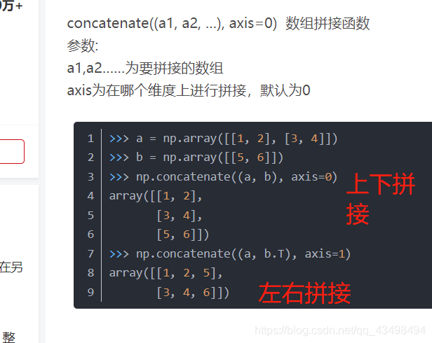
df1=pd.Series(np.random.rand(4)*3,index=['a','b','c','d'], name='series')
#所以必须randn有可能生成负数值就画不出饼状图了。所以应该是rand
#np.random.rand(d0,d1,d2……dn)
# 注:使用方法与np.random.randn()函数相同
# 通过本函数可以返回一个或一组服从“0~1”均匀分布的随机样本值。随机样本取值范围是[0,1),不包括1。
# 应用:在深度学习的Dropout正则化方法中,可以用于生成dropout随机向量(dl),例如(keep_prob表示保留神经元的比例):dl = np.random.rand(al.shape[0],al.shape[1]) < keep_prob
print(df1)
#1画饼图
print(df1.plot.pie())
plt.show()#每次一个这个就会出来一个画布
#2指定类似正方形的饼图,为列标签abcd指定名字,显示百分比,设置字体为20,以及指定颜色
print(df1.plot.pie(figsize=(6,6),labels=['AA','BB','CC','DD'],autopct='%0.2f',fontsize=20,colors=['r','g','b','c']))
# #散布图在数据很大时,可以直接观察数据之间的关联关系,甚至一些分类。
# #1将x轴用a,b作为y轴
# print(df1.plot.scatter(x='a',y='b'))
plt.show()
结果;
a 1.711469
b 0.155807
c 0.171055
d 2.532418
Name: series, dtype: float64
AxesSubplot(0.22375,0.11;0.5775x0.77)
AxesSubplot(0.1275,0.11;0.77x0.77)

七、股票数据分析
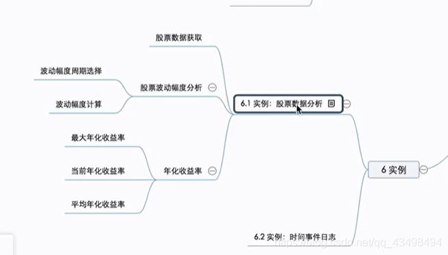

股票数据分析数据说明:参考以下网址:
https://github.com/kamidox/stock-analysis (https://github.com/kamidox/stock-analysis)

股票分析代码
import numpy as np
import pandas as pd
import matplotlib.pyplot as plt
#一般我们希望股票波动大一些,这样获取收益多,对选股有参考意义。
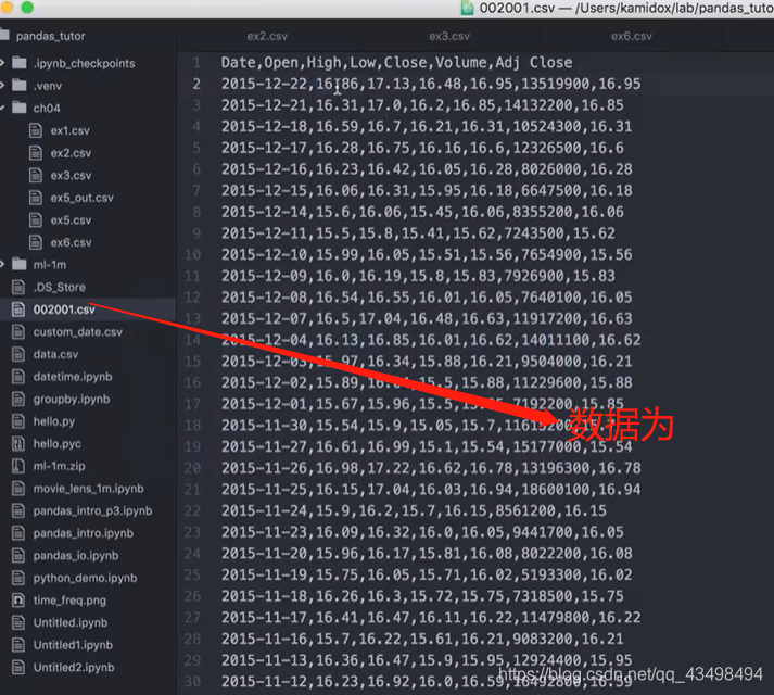
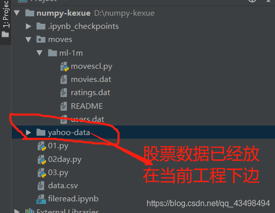
#1将股票数据读进来,指定将第一列作为索引,且将日期解析出来parse_dates=True,默认不解析日期,日期仍是字符串
da1=pd.read_csv('600690.csv',index_col='Date',parse_dates=True)
print(da1)
#2我们更关心Adj Close这列数据
da2=da1['Adj Close']
print(da2)
#3因为我们关心这个Adj Close数据的波动,所以对他按月m或M都行重采样,T是按照分钟采样
#重采样后将Adj Close数据按照每个月分成一个开盘价,最高最低价,收盘价就是如11月的最后一天的价格就是作为11月的收盘价
da3=da2.resample('m',how='ohlc')
print(da3)
#4股票的波动就是最高价格减去最低价格,可以看到11月波动幅度为0.077=7%
da4=(da3.high-da3.low)/da3.low
#5求个平均值,每个月波动幅度大概是17%
print(da4.mean())
#6看一下近20年股票Adj Close变化
print(da2.plot(figsize=(8,6)))
plt.show()#这是一个画布
#看一下Adj Close最大变化幅度,从最低价格到最高价格增加大约1110元
da5=(da2.max()-da2.min())/da2.min()
print(da5)
print(9.14000/0.05072)
#7看股票最早买da2.iloc[-1]以及到现在da2.iloc[0]第一个索引对应的值的增加了多少倍,总增长幅度
da6=da2.iloc[0]/da2.iloc[-1]
da7=da2.index[-1]#最早日期1993
da8=da2.index[0]#现在日期 2016
print(da7.year,da8.year)
#8年增长幅度,相当于对da6总增长幅度,开20次方,就基本是每年增长幅度,大概就是1.253.-1=0.253
da9=da6**(1.0/(da8.year-da7.year))
print(da9)
#9da2是时间戳为索引的序列,转化为以时期为索引的序列,A就是年为单位,此时就是年数据了。
da10=da2.to_period('A')
print(da10)
#10将年数据按照索引日期进行分组,first就是将分组后的每年的第一天的数据显示出来了
da11=da10.groupby(level=0).first()
print(da11)
#11将数据da11画出来,可以看到走势图了。
print(da11.plot())
plt.show()#这也是一个画布
#12用da11进行每年都是这一年数据减去上一年数据的结果,可以看到每年对于上一年是增加还是减少
#1993年前面没值,所以NaN,1994就是1994-1993的值
diff=da11.diff()
print(diff)
#13计算每年相对于上一年的增长情况如:1994-1993/1993
da=diff/(da11-diff)#这样除的是94年数据,应该除以93年数据,因为diff是1994-1993=diff的数据。
# 所以要得到93数据就是94-diff,而da11.index就是94,95,96等的数据了,所以直接减去diff即可
print(da)#可以看到94相对93下跌了0.311约为31%
#14画出da图像柱状图,可以看到98年是跌的
print(da.plot(kind='bar'))
plt.show()
结果:
D:\ProgramData\Anaconda3\python.exe D:/numpy-kexue/yahoo-data/gpanalysisi.py
Open High Low Close Volume Adj Close
Date
2016-05-20 8.74000 9.15000 8.74000 9.14000 55390400 9.14000
2016-05-19 8.84000 9.05000 8.81000 8.84000 34785900 8.84000
2016-05-18 8.82000 8.93000 8.65000 8.88000 44254300 8.88000
2016-05-17 9.08000 9.08000 8.82000 8.83000 42392200 8.83000
2016-05-16 8.90000 9.08000 8.80000 9.07000 59749500 9.07000
2016-05-13 9.00000 9.08000 8.86000 8.98000 67999000 8.98000
2016-05-12 9.04000 9.39000 8.82000 9.07000 90370400 9.07000
2016-05-11 8.68000 9.38000 8.63000 9.11000 134761600 9.11000
2016-05-10 8.25000 8.83000 8.17000 8.66000 86509000 8.66000
2016-05-09 8.30000 8.38000 8.08000 8.25000 32951400 8.25000
2016-05-06 8.70000 8.72000 8.32000 8.33000 34623000 8.33000
2016-05-05 8.64000 8.69000 8.55000 8.66000 26526000 8.66000
2016-05-04 8.66000 8.83000 8.61000 8.64000 40301300 8.64000
2016-05-03 8.34000 8.85000 8.28000 8.71000 99180100 8.71000
2016-05-02 8.33000 8.33000 8.33000 8.33000 0 8.33000
2016-04-29 8.00000 8.53000 7.91000 8.33000 55185500 8.33000
2016-04-28 7.89000 8.00000 7.85000 8.00000 22526400 8.00000
2016-04-27 7.92000 7.94000 7.87000 7.89000 19604900 7.89000
2016-04-26 7.99000 7.99000 7.85000 7.91000 21428000 7.91000
2016-04-25 8.00000 8.02000 7.90000 7.96000 15823900 7.96000
2016-04-22 7.97000 8.06000 7.94000 8.00000 17039000 8.00000
2016-04-21 8.08000 8.10000 7.98000 7.99000 19608500 7.99000
2016-04-20 8.34000 8.35000 7.83000 8.11000 35343900 8.11000
2016-04-19 8.30000 8.35000 8.27000 8.33000 11355800 8.33000
2016-04-18 8.35000 8.38000 8.28000 8.29000 20101300 8.29000
2016-04-15 8.46000 8.46000 8.38000 8.41000 20774900 8.41000
2016-04-14 8.45000 8.46000 8.38000 8.44000 20479200 8.44000
2016-04-13 8.41000 8.52000 8.39000 8.41000 47563700 8.41000
2016-04-12 8.40000 8.49000 8.33000 8.38000 14814200 8.38000
2016-04-11 8.33000 8.51000 8.33000 8.44000 18856000 8.44000
... ... ... ... ... ... ...
1993-12-30 8.90006 9.07999 8.87997 8.91003 4438400 0.03534
1993-12-29 9.29996 9.38002 8.87997 8.95006 6330800 0.03549
1993-12-28 9.54001 9.61994 9.11005 9.24996 6950800 0.03668
1993-12-27 9.49998 9.70000 9.44998 9.52006 4139200 0.03776
1993-12-24 9.65000 9.80001 9.35994 9.49998 5540900 0.03768
1993-12-23 10.10004 10.10004 9.49998 9.60996 6270100 0.03811
1993-12-22 9.44998 10.30006 9.39997 9.45995 25474100 0.03752
1993-12-21 9.04994 9.38002 9.00007 9.32004 15368000 0.03696
1993-12-20 9.80001 10.00003 8.24999 8.96004 18951900 0.03553
1993-12-17 10.79997 11.10000 10.78002 10.84998 8491300 0.04303
1993-12-16 11.36000 11.68995 11.01994 11.10000 9199000 0.04402
1993-12-15 11.27994 11.40003 10.74997 11.30002 10883800 0.04481
1993-12-14 11.70006 11.98998 11.20001 11.30002 11307000 0.04481
1993-12-13 12.38005 12.39999 11.81004 11.89994 8781100 0.04719
1993-12-10 12.29998 12.67994 11.94995 12.28004 14234500 0.04870
1993-12-09 12.70002 12.71997 12.01006 12.19997 12680400 0.04838
1993-12-08 12.80003 12.85004 12.28004 12.70002 19528800 0.05037
1993-12-07 13.05006 13.15007 12.67994 12.75003 22959100 0.05056
1993-12-06 13.19994 13.38998 12.90004 12.96002 20992600 0.05140
1993-12-03 13.00005 13.47004 12.90004 13.15007 40884000 0.05215
1993-12-02 13.05006 13.07998 12.90004 13.00005 15753500 0.05156
1993-12-01 13.34995 13.39996 12.91002 13.07998 20024800 0.05187
1993-11-30 13.39996 13.47004 13.15007 13.22002 22483300 0.05243
1993-11-29 13.19994 13.54997 12.90004 13.17999 28609200 0.05227
1993-11-26 14.20003 14.25004 13.10006 13.34995 59775300 0.05294
1993-11-25 13.29995 14.40005 13.28000 13.78005 130913000 0.05465
1993-11-24 12.80003 13.69999 12.50000 13.01003 102888700 0.05160
1993-11-23 13.10006 13.17999 12.50000 12.80003 68880000 0.05076
1993-11-22 12.96999 13.34995 12.67994 13.00005 126529800 0.05156
1993-11-19 11.99995 12.90004 11.91005 12.79006 355926800 0.05072
[5847 rows x 6 columns]
Date
2016-05-20 9.14000
2016-05-19 8.84000
2016-05-18 8.88000
2016-05-17 8.83000
2016-05-16 9.07000
2016-05-13 8.98000
2016-05-12 9.07000
2016-05-11 9.11000
2016-05-10 8.66000
2016-05-09 8.25000
2016-05-06 8.33000
2016-05-05 8.66000
2016-05-04 8.64000
2016-05-03 8.71000
2016-05-02 8.33000
2016-04-29 8.33000
2016-04-28 8.00000
2016-04-27 7.89000
2016-04-26 7.91000
2016-04-25 7.96000
2016-04-22 8.00000
2016-04-21 7.99000
2016-04-20 8.11000
2016-04-19 8.33000
2016-04-18 8.29000
2016-04-15 8.41000
2016-04-14 8.44000
2016-04-13 8.41000
2016-04-12 8.38000
2016-04-11 8.44000
...
1993-12-30 0.03534
1993-12-29 0.03549
1993-12-28 0.03668
1993-12-27 0.03776
1993-12-24 0.03768
1993-12-23 0.03811
1993-12-22 0.03752
1993-12-21 0.03696
1993-12-20 0.03553
1993-12-17 0.04303
1993-12-16 0.04402
1993-12-15 0.04481
1993-12-14 0.04481
1993-12-13 0.04719
1993-12-10 0.04870
1993-12-09 0.04838
1993-12-08 0.05037
1993-12-07 0.05056
1993-12-06 0.05140
1993-12-03 0.05215
1993-12-02 0.05156
1993-12-01 0.05187
1993-11-30 0.05243
1993-11-29 0.05227
1993-11-26 0.05294
1993-11-25 0.05465
1993-11-24 0.05160
1993-11-23 0.05076
1993-11-22 0.05156
1993-11-19 0.05072
Name: Adj Close, Length: 5847, dtype: float64
D:/numpy-kexue/yahoo-data/gpanalysisi.py:21: FutureWarning: how in .resample() is deprecated
the new syntax is .resample(...).ohlc()
da3=da2.resample('m',how='ohlc')
open high low close
Date
1993-11-30 0.05072 0.05465 0.05072 0.05243
1993-12-31 0.05187 0.05215 0.03534 0.03573
1994-01-31 0.03768 0.03926 0.03331 0.03331
1994-02-28 0.03232 0.03573 0.03232 0.03331
1994-03-31 0.03300 0.03522 0.02915 0.03125
1994-04-30 0.03125 0.03125 0.02109 0.02346
1994-05-31 0.02346 0.02480 0.02088 0.02129
1994-06-30 0.02114 0.02114 0.01717 0.01727
1994-07-31 0.01681 0.01701 0.01397 0.01418
1994-08-31 0.01804 0.03501 0.01727 0.03501
1994-09-30 0.03542 0.04532 0.03119 0.03119
1994-10-31 0.03119 0.03119 0.02475 0.02485
1994-11-30 0.02614 0.02877 0.02578 0.02635
1994-12-31 0.02629 0.02665 0.02449 0.02459
1995-01-31 0.02459 0.02609 0.02165 0.02253
1995-02-28 0.02253 0.02403 0.02155 0.02217
1995-03-31 0.02227 0.02774 0.02227 0.02681
1995-04-30 0.02712 0.02712 0.02227 0.02274
1995-05-31 0.02274 0.03583 0.02274 0.02681
1995-06-30 0.02702 0.02805 0.02454 0.02454
1995-07-31 0.02475 0.08573 0.02475 0.08573
1995-08-31 0.09100 0.09809 0.08606 0.09067
1995-09-30 0.09199 0.09776 0.09018 0.09249
1995-10-31 0.09249 0.10386 0.09084 0.09760
1995-11-30 0.09776 0.10007 0.08540 0.08540
1995-12-31 0.08408 0.08457 0.07254 0.07254
1996-01-31 0.07254 0.07781 0.06974 0.07781
1996-02-29 0.07699 0.08161 0.07336 0.08161
1996-03-31 0.08161 0.08985 0.08161 0.08161
1996-04-30 0.08210 0.12084 0.08128 0.10864
... ... ... ... ...
2013-12-31 7.54922 9.24802 7.54922 8.85739
2014-01-31 8.85739 9.90211 8.14426 9.62049
2014-02-28 9.62049 10.15193 8.05795 8.28961
2014-03-31 8.43950 8.43950 6.95419 7.37662
2014-04-30 7.38116 7.86264 6.81792 6.97236
2014-05-31 6.97236 6.97236 6.27285 6.83609
2014-06-30 6.83609 7.13133 6.65440 7.12916
2014-07-31 6.97942 7.86332 6.63649 7.82951
2014-08-31 7.87781 8.08068 7.33685 7.69910
2014-09-30 7.74257 8.27871 7.63148 7.63148
2014-10-31 7.63148 7.98408 7.43345 7.98408
2014-11-30 8.04687 8.55885 7.83434 8.26422
2014-12-31 8.46225 9.37513 8.46225 8.96458
2015-01-31 8.96458 10.25903 8.96458 9.63595
2015-02-28 9.50554 9.93059 9.20125 9.87263
2015-03-31 9.92093 12.48085 9.35098 12.48085
2015-04-30 12.56780 13.99266 12.52432 13.09427
2015-05-31 13.09427 15.18085 12.36010 14.17620
2015-06-30 14.87173 15.55277 13.05080 14.64955
2015-07-31 13.67388 15.09874 6.99150 11.18000
2015-08-31 11.37000 12.31000 8.61000 10.04000
2015-09-30 10.11000 10.35000 9.03000 9.06000
2015-10-31 9.06000 9.92000 9.06000 9.92000
2015-11-30 9.92000 9.92000 9.92000 9.92000
2015-12-31 9.92000 9.92000 9.92000 9.92000
2016-01-31 9.92000 9.92000 9.92000 9.92000
2016-02-29 8.93000 8.93000 7.48000 7.48000
2016-03-31 8.23000 8.92000 8.23000 8.47000
2016-04-30 8.55000 8.59000 7.89000 8.33000
2016-05-31 8.33000 9.14000 8.25000 9.14000
[271 rows x 4 columns]
0.1765642638938196
AxesSubplot(0.125,0.2;0.775x0.68)
1112.2977809591985
180.205047318612
1993 2016
1.2533628673066715
Date
2016 9.14000
2016 8.84000
2016 8.88000
2016 8.83000
2016 9.07000
2016 8.98000
2016 9.07000
2016 9.11000
2016 8.66000
2016 8.25000
2016 8.33000
2016 8.66000
2016 8.64000
2016 8.71000
2016 8.33000
2016 8.33000
2016 8.00000
2016 7.89000
2016 7.91000
2016 7.96000
2016 8.00000
2016 7.99000
2016 8.11000
2016 8.33000
2016 8.29000
2016 8.41000
2016 8.44000
2016 8.41000
2016 8.38000
2016 8.44000
...
1993 0.03534
1993 0.03549
1993 0.03668
1993 0.03776
1993 0.03768
1993 0.03811
1993 0.03752
1993 0.03696
1993 0.03553
1993 0.04303
1993 0.04402
1993 0.04481
1993 0.04481
1993 0.04719
1993 0.04870
1993 0.04838
1993 0.05037
1993 0.05056
1993 0.05140
1993 0.05215
1993 0.05156
1993 0.05187
1993 0.05243
1993 0.05227
1993 0.05294
1993 0.05465
1993 0.05160
1993 0.05076
1993 0.05156
1993 0.05072
Freq: A-DEC, Name: Adj Close, Length: 5847, dtype: float64
Date
1993 0.03573
1994 0.02459
1995 0.07254
1996 0.27879
1997 0.69135
1998 0.50219
1999 0.48011
2000 0.80252
2001 0.78662
2002 0.53786
2003 0.60910
2004 0.56913
2005 0.60712
2006 1.50079
2007 3.80700
2008 1.67358
2009 4.82062
2010 5.76779
2011 3.70347
2012 5.72073
2013 8.85739
2014 8.96458
2015 9.92000
2016 9.14000
Freq: A-DEC, Name: Adj Close, dtype: float64
AxesSubplot(0.125,0.11;0.775x0.77)
Date
1993 NaN
1994 -0.01114
1995 0.04795
1996 0.20625
1997 0.41256
1998 -0.18916
1999 -0.02208
2000 0.32241
2001 -0.01590
2002 -0.24876
2003 0.07124
2004 -0.03997
2005 0.03799
2006 0.89367
2007 2.30621
2008 -2.13342
2009 3.14704
2010 0.94717
2011 -2.06432
2012 2.01726
2013 3.13666
2014 0.10719
2015 0.95542
2016 -0.78000
Freq: A-DEC, Name: Adj Close, dtype: float64
Date
1993 NaN
1994 -0.311783
1995 1.949980
1996 2.843259
1997 1.479824
1998 -0.273610
1999 -0.043967
2000 0.671534
2001 -0.019813
2002 -0.316239
2003 0.132451
2004 -0.065621
2005 0.066751
2006 1.471982
2007 1.536664
2008 -0.560394
2009 1.880424
2010 0.196483
2011 -0.357905
2012 0.544695
2013 0.548297
2014 0.012102
2015 0.106577
2016 -0.078629
Freq: A-DEC, Name: Adj Close, dtype: float64
AxesSubplot(0.125,0.11;0.775x0.77)
Process finished with exit code 0
八、时间事件日志
注:就是记录自己以往的信息的日志,如消费, 就可以记录过去一段时间的消费情况,从而进行分析,为以后消费做参考。也可以自己过去时间都花在那些地方了。对时间做理性分析。
介绍个工具: 好用工具:
好用工具:


导出时间日志步骤:


下图中文件前三行是文档说明,读取文件,可以不需要读出来。
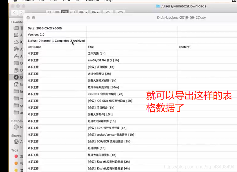
时间日志文件分析


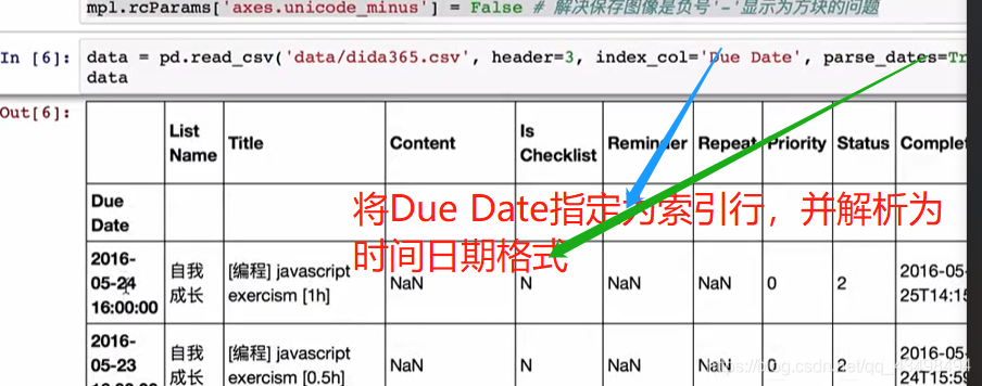
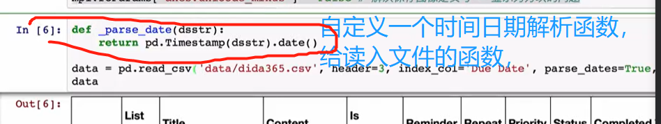

1是没有按时完成,但是完成了。对于0未完成的事情我们不关心,要过滤掉。
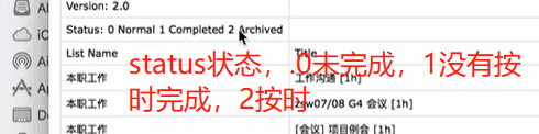
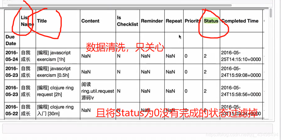
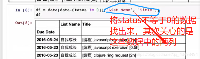


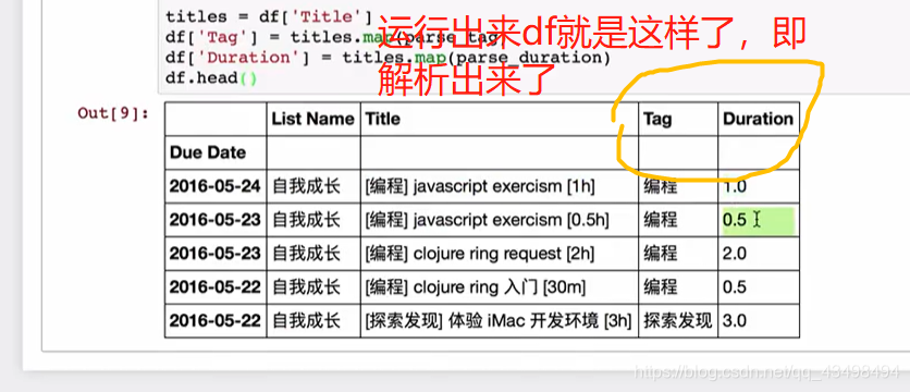


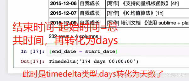
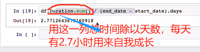
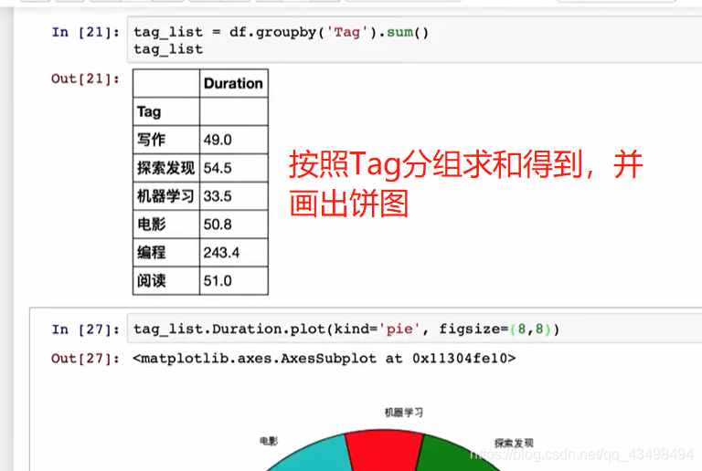

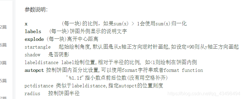


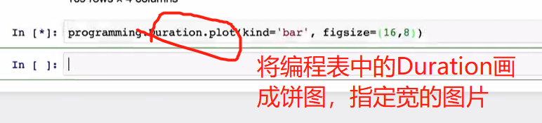
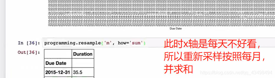
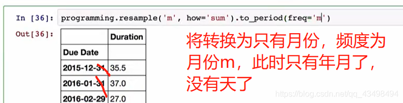
以下是用柱状图分析编程每月所分配的时间情况。


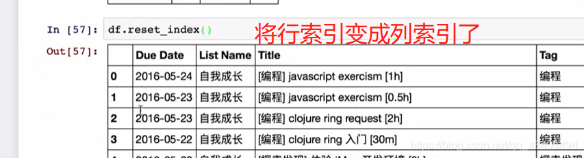

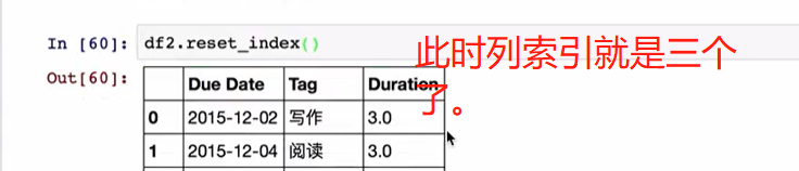


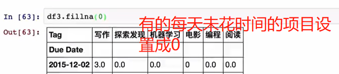

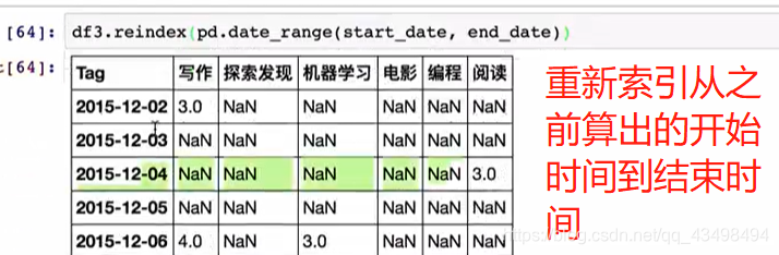
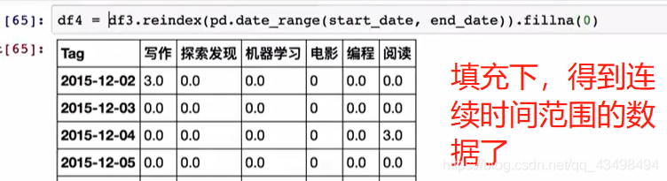
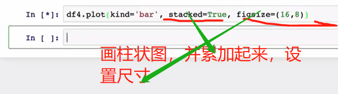

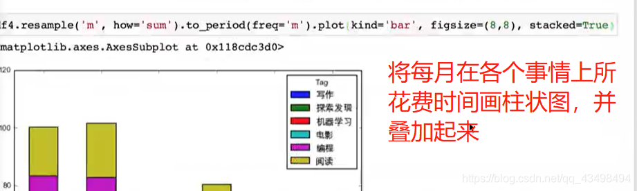
九、pandas教程课程小结