均匀分布
- 如图:
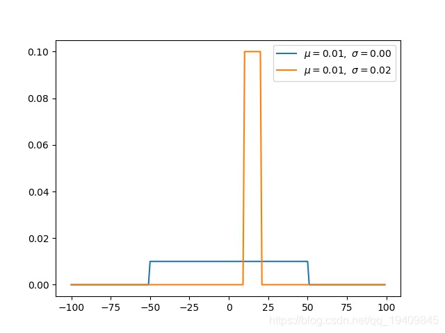
- 代码如下:
def uniform(x, a, b):
    y = [1 / (b - a) if a <= val and val <= b
         else 0 for val in x]
    return x, y, np.mean(y), np.std(y)
x = np.arange(-100, 100)  # define range of x
for ls in [(-50, 50), (10, 20)]:
    a, b = ls[0], ls[1]
    x, y, u, s = uniform(x, a, b)
    plt.plot(x, y, label=r'$\mu=%.2f,\ \sigma=%.2f$' % (u, s))
plt.legend()
plt.title('均匀分布(连续)')
plt.savefig(image_file_path+'/uniform.jpg')
plt.show()
伯努利分布(离散)
- 如图:
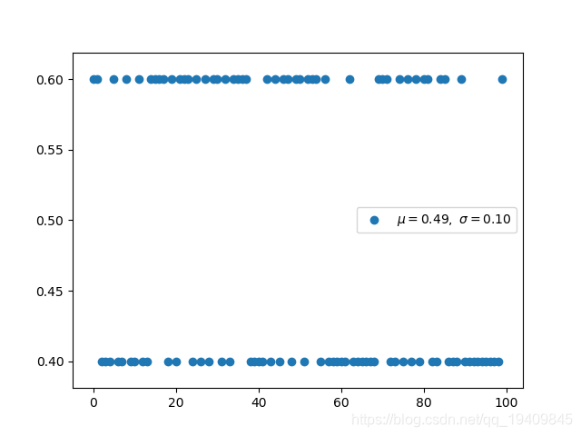
- 代码如下
def bernoulli(p, k):
    return p if k else 1 - p
n_experiment = 100
p = 0.6
x = np.arange(n_experiment)
y = []
for _ in range(n_experiment):
    pick = bernoulli(p, k=bool(random.getrandbits(1)))
    y.append(pick)

u, s = np.mean(y), np.std(y)
plt.scatter(x, y, label=r'$\mu=%.2f,\ \sigma=%.2f$' % (u, s))
plt.legend()
plt.title('伯努利分布(离散)')
plt.savefig(image_file_path+'/bernoulli.png')
plt.show()
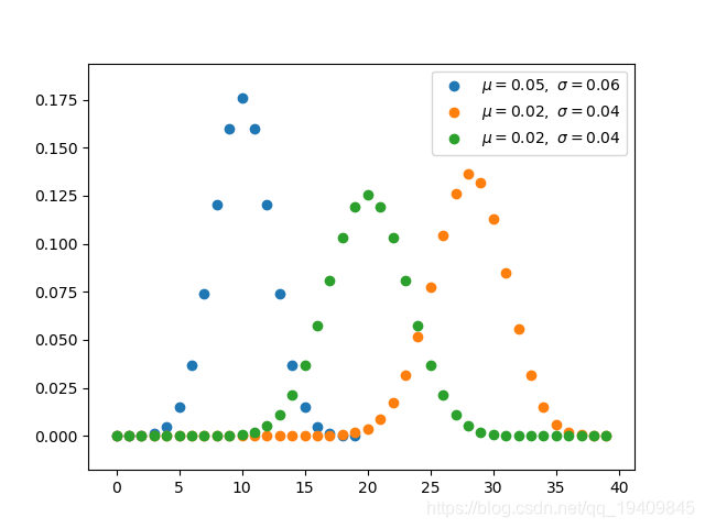
二项分布(离散)
-
如图:
-
代码如下:
def const(n, r):
    r = min(r, n - r)
    numer = reduce(op.mul, range(n, n - r, -1), 1)
    denom = reduce(op.mul, range(1, r + 1), 1)
    return numer / denom

def binomial(n, p):
    q = 1 - p
    y = [const(n, k) * (p ** k) * (q ** (n - k)) for k in range(n)]
    return y, np.mean(y), np.std(y)

for ls in [(0.5, 20), (0.7, 40), (0.5, 40)]:
    p, n_experiment = ls[0], ls[1]
    x = np.arange(n_experiment)
    y, u, s = binomial(n_experiment, p)
    plt.scatter(x, y, label=r'$\mu=%.2f,\ \sigma=%.2f$' % (u, s))

plt.legend()
plt.title('二项分布(离散)')
plt.savefig(image_file_path+'/binomial.png')

plt.show()
多项式分布(离散)
- 如图:
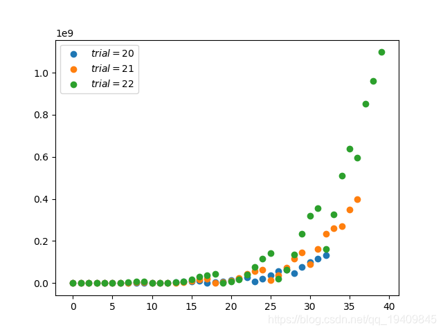
- 代码如下:
def factorial(n):
    return reduce(op.mul, range(1, n + 1), 1)

def const(n, a, b, c):
    assert a + b + c == n
    numer = factorial(n)
    denom = factorial(a) * factorial(b) * factorial(c)
    return numer / denom

def multinomial(n):
    ls = []
    for i in range(1, n + 1):
        for j in range(i, n + 1):
            for k in range(j, n + 1):
                if i + j + k == n:
                    ls.append([i, j, k])

    y = [const(n, l[0], l[1], l[2]) for l in ls]
    x = np.arange(len(y))
    return x, y, np.mean(y), np.std(y)

for n_experiment in [20, 21, 22]:
    x, y, u, s = multinomial(n_experiment)
    plt.scatter(x, y, label=r'$trial=%d$' % (n_experiment))

plt.legend()
plt.title('多项式分布(离散)')
plt.savefig(image_file_path+'/multinomial.png')
plt.show()
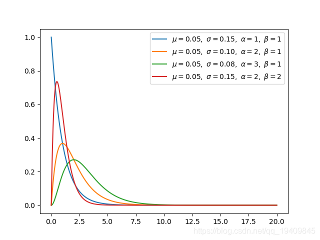
伽马分布(连续)
- 如图:
- 代码如下:
def gamma_function(n):
    cal = 1
    for i in range(2, n):
        cal *= i
    return cal

def gamma(x, a, b):
    c = (b ** a) / gamma_function(a)
    y = c * (x ** (a - 1)) * np.exp(-b * x)
    return x, y, np.mean(y), np.std(y)

for ls in [(1, 1), (2, 1), (3, 1), (2, 2)]:
    a, b = ls[0], ls[1]
    x = np.arange(0, 20, 0.01, dtype=np.float)
    x, y, u, s = gamma(x, a=a, b=b)
    plt.plot(x, y, label=r'$\mu=%.2f,\ \sigma=%.2f,'

                         r'\ \alpha=%d,\ \beta=%d$' % (u, s, a, b))

plt.legend()
plt.title('伽马分布(连续)')
plt.savefig(image_file_path+'/gamma.png')
plt.show()
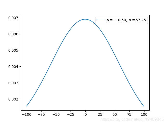
高斯分布(连续)
- 如图:
- 代码如下:
    def gaussian(x, n):
        u = x.mean()

        s = x.std()

        # divide [x.min(), x.max()] by n

        x = np.linspace(x.min(), x.max(), n)

        a = ((x - u) ** 2) / (2 * (s ** 2))

        y = 1 / (s * np.sqrt(2 * np.pi)) * np.exp(-a)

        return x, y, x.mean(), x.std()

    x = np.arange(-100, 100)  # define range of x

    x, y, u, s = gaussian(x, 10000)

    plt.plot(x, y, label=r'$\mu=%.2f,\ \sigma=%.2f$' % (u, s))

    plt.legend()
    plt.title('高斯分布(连续)')
    plt.savefig(image_file_path+'/gaussian.png')

    plt.show()
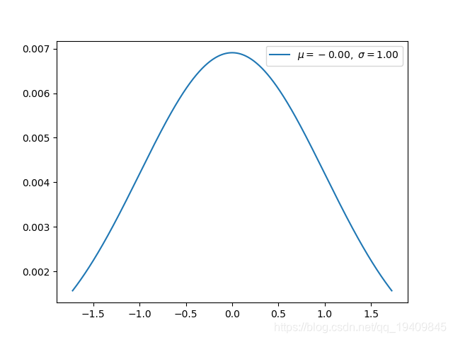
正态分布(连续)
- 如图:
- 代码如下:
def normal(x, n):
    u = x.mean()

    s = x.std()

    # normalization

    x = (x - u) / s

    # divide [x.min(), x.max()] by n

    x = np.linspace(x.min(), x.max(), n)

    a = ((x - 0) ** 2) / (2 * (1 ** 2))

    y = 1 / (s * np.sqrt(2 * np.pi)) * np.exp(-a)

    return x, y, x.mean(), x.std()

x = np.arange(-100, 100)  # define range of x

x, y, u, s = normal(x, 10000)

plt.plot(x, y, label=r'$\mu=%.2f,\ \sigma=%.2f$' % (u, s))

plt.legend()
plt.title('正态分布(连续)')
plt.savefig(image_file_path+'/normal.png')

plt.show()
