“Capital Management” As this section demonstrates, depending on the strategy characteristics and the trading capital available, the Kelly criterion helps with sizing the trades.
“ML-Based Trading Strategy” To gain confidence in an algorithmic trading strategy, the strategy needs to be backtested thoroughly both with regard to performance and risk characteristics; the example strategy used is based on a classification algorithm from machine learning as introduced in 11_15TradingStrategies
(https://blog.csdn.net/Linli522362242/article/details/102314389,
https://blog.csdn.net/Linli522362242/article/details/102559594).
“Online Algorithm” To deploy the algorithmic trading strategy for automated trading, it needs to be translated into an online algorithm that works with incoming streaming data in real time.
“Infrastructure and Deployment” To run automated algorithmic trading strategies robustly and reliably, deployment in the cloud is the preferred option from an availability, performance, and security point of view.
“Logging and Monitoring” To be able to analyze the history and certain events during the deployment of an automated trading strategy, logging plays an important role; monitoring via socket communication allows one to observe events (remotely) in real time.
Capital Management A central question in algorithmic trading is how much capital to deploy to a given algorithmic trading strategy given the total available capital. The answer to this question depends on the main goal one is trying to achieve by algorithmic trading. Most individuals and financial institutions will agree that the maximization of long-term wealth is a good candidate objective. This is what Edward Thorpe had in mind when he derived the Kelly criterion for investing, as described in the paper by Rotando and Thorp (1992).
###############################################################################
在机率论中,凯利公式(也称凯利方程式)是一个用以使特定赌局中,拥有正期望值之重复行为长期增长率最大化的公式,由约翰·拉里·凯利於 1956 年在《贝尔系统技术期刊》中发表,可用以计算出每次游戏中应投注的资金比例。
除可将长期增长率最大化外,此方程式不允许在任何赌局中,有失去全部现有资金的可能,因此有不存在破产疑虑的优点。方程式假设货币与赌局可无穷分割,而只要资金足够多,在实际应用上不成问题。凯利公式的最一般性陈述为,藉由寻找能最大化结果对数期望值的资本比例 f*,即可获得长期增长率的最大化。
对于只有两种结果,即输去所有资金,或者获得资金乘以特定赔率的彩金的简单赌局而言,可由一般性陈述导出以下式子:
![]()
其中,f* 为现有资金应进行下次投注的比例;b 为投注可得的赔率(此处的赔率是净赔率);p 为获胜率;q 为落败率,即 1 - p。
举例而言,若一赌博有 40% 的获胜率(p = 0.4,q = 0.6),而赌客在赢得赌局时,可获得二对一的赔率(b = 2),则赌客应在每次机会中下注现有资金的 10%(f* = 0.1),以最大化资金的长期增长率。
the value of b in the following example is 1 .
注意,这个广为人知的公式只适用于牌桌赌博,即输的情况下本金全部亏光,而适用更为广泛的凯利公式是:
其中f*,p,q同上,rW是获胜后的净赢率,rL是净损失率。换句话说,第一个公式是第二个公式里rL=100%的特例。
###############################################################################
The Kelly Criterion in a Binomial Setting
The common way of introducing the theory of the Kelly criterion for investing is on the basis of a coin
tossing game, or more generally a binomial setting (where only two outcomes are possible). This
section follows that route. Assume a gambler is playing a coin tossing game against an infinitely rich
bank or casino. Assume further that the probability for heads is some value p for which![]() < p < 1
< p < 1
holds. Probability for tails is defined by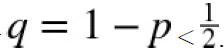 The gambler can place bets b > 0 of
arbitrary size, whereby the gambler wins the same amount if right and loses it all if wrong. Given the
assumptions about the probabilities, the gambler would of course want to bet on heads. Therefore, the
expected value for this betting game![]() (i.e., the random variable representing this game) in a oneshot
(i.e., the random variable representing this game) in a oneshot
setting is:
A risk-neutral gambler with unlimited funds would like to bet as large an amount as possible since
this would maximize the expected payoff. However, trading in financial markets is not a one-shot
game in general. It is a repeated one. Therefore, ![]() assume that represents the amount that is bet on
assume that represents the amount that is bet on
day i and that ![]() represents the initial capital (
represents the initial capital (![]() is from
is from ![]() ). The capital
). The capital ![]() at the end of day one depends on the
at the end of day one depends on the
betting success(win b or lose b) on that day and might be ![]() . The expected value for a gamble
. The expected value for a gamble
that is repeated n times then is:
In classical economic theory, with risk-neutral, expected utility-maximizing agents, a gambler would
try to maximize this expression. It is easily seen that it is maximized by betting all available funds —
i.e., ![]() (Ci-2 + bi-1 or Ci-2 - bi-1)— like in the one-shot scenario. However, this in turn implies that a single loss will wipe out all available funds and will lead to ruin (unless unlimited borrowing is possible).
(Ci-2 + bi-1 or Ci-2 - bi-1)— like in the one-shot scenario. However, this in turn implies that a single loss will wipe out all available funds and will lead to ruin (unless unlimited borrowing is possible).
Therefore, this strategy does not lead to a maximization of long-term wealth.
While betting the maximum capital available might lead to sudden ruin, betting nothing at all avoids
any kind of loss but does not benefit from the advantageous gamble either. This is where the Kelly
criterion comes into play, since it derives the optimal fraction ![]() of the available capital to bet per
of the available capital to bet per
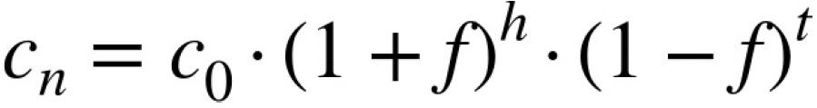
round of betting. Assume that n = h + t, where h stands for the number of heads observed during n
rounds of betting and where t stands for the number of tails. With these definitions, the available
capital after n rounds is:
In such a context, long-term wealth maximization boils down to maximizing the average geometric
growth rate per bet, which is given as: Note growth rate=![]()

The problem then formally is to maximize the expected average rate of growth![]() by choosing f
by choosing f
optimally. With ![]() and
and ![]() , one gets:
, one gets:

One can now maximize the term by choosing the optimal fraction![]() according to the first-order
according to the first-order
condition. The first derivative (the first derivative of log(x) is 1/x)is given by: Note p+q =1

From the first-order condition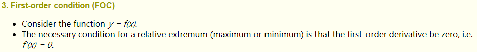 , one gets:
G ' ( f ) = 0 ⇒ f * = p - q
If one trusts this to be the maximum (and not the minimum), this result implies that it is optimal to
invest a fraction f * = p - q per round of betting. With, for example, p = 0.55 one has f * = 0.55 - 0.45
= 0.1, indicating that the optimal fraction is 10%.
The following Python code formalizes these concepts and results through simulation. First, some
imports and configurations:
import math
import time
import numpy as np
import pandas as pd
import datetime as dt
import cufflinks as cf
from pylab import plt
np.random.seed(1000)
plt.style.use('seaborn')
%matplotlib inline
The idea is to simulate, for example, 50 series with 100 coin tosses per series. The Python code for this is straightforward:
p =0.55 #Fixes the probability for heads.
f=p-(1-p) #Calculates the optimal fraction according to the Kelly criterion.
f
![]()
I=50 #The number of series to be simulated.
n=100 #The number of trials per series.
The major part is the Python function run_simulation(), which achieves the simulation according to the prior assumptions. Figure shows the simulation results:
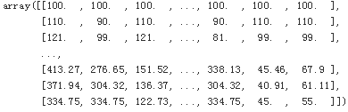
def run_simulation(f):
#(100,50)
c = np.zeros((n,I)) #Instantiates an ndarray object to store the simulation results.
c[0] =100 #fill first row with all zeros #Initializes the starting capital with 100.
for i in range(I): #Outer loop for the series simulations. #paths
for t in range(1,n): #Inner loop for the series itself. #times
o = np.random.binomial(1,p) #Simulates the tossing of a coin.
if o>0 : #If 1, i.e., heads
c[t,i] = (1+f)*c[t-1,i] #then add the win to the capital.
else: #If 0, i.e., tails
c[t,i] = (1-f)*c[t-1,i] #then subtract the loss from the capital.
return c
c_1 = run_simulation(f) #Runs the simulation. #f=0.1
c_1.round(2)
plt.figure(figsize=(10,6))
plt.plot(c_1, 'b', lw=0.5)
plt.plot(c_1.mean(axis=1),'r',lw=2.5)
plt.title('50 simulated series with 100 trials each (red line = average)')

The following code repeats the simulation for different values of f. As shown in Figure.a lower fraction leads to a lower growth rate on average. Higher values might lead to a higher average capital at the end of the simulation (f = 0.25) or to a much lower average capital (f = 0.5). In both cases where the fraction f is higher, the volatility increases considerably:
c_2 = run_simulation(0.05) #Simulation with f = 0.05.
c_3 = run_simulation(0.25) #Simulation with f = 0.25.
c_4 = run_simulation(0.5) #Simulation with f = 0.5.

plt.figure(figsize=(10,6))
plt.plot(c_4.mean(axis=1),'k',label='$f=0.5$')
plt.plot(c_3.mean(axis=1),'y',label='$f=0.25$')
plt.plot(c_1.mean(axis=1),'r',label='$f^*=0.1$')
plt.plot(c_2.mean(axis=1),'b',label='$f=0.05$')
plt.legend(loc=0)
plt.title('Average capital over time for different fractions')

a lower fraction(f=0.05 or f=0.1) leads to a lower growth rate on average.
Higher values(f) might lead to a higher average capital at the end of the simulation (f = 0.25)
or to a much lower average capital (f = 0.5).
Kelly Criterion for Stocks and Indices
Assume now a stock market setting in which the relevant stock (index) can take on only two values after a period of one year from today, given its known value today. The setting is again binomial, but this time a bit closer on the modeling side to stock market realities. Specifically, assume that:
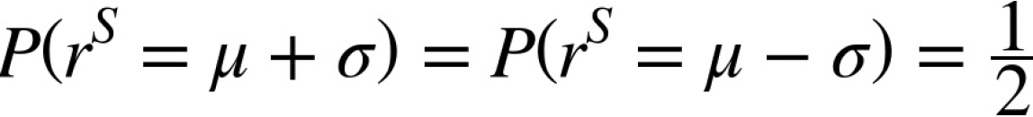
with ![]() being the expected return of the stock over one year and
being the expected return of the stock over one year and
![]() being the standard deviation of returns (volatility). In a one-period setting, one gets for the available capital
being the standard deviation of returns (volatility). In a one-period setting, one gets for the available capital
after one year (with ![]() and f defined as before): Note:
and f defined as before): Note: ![]() the return of the stock, equal to
the return of the stock, equal to 
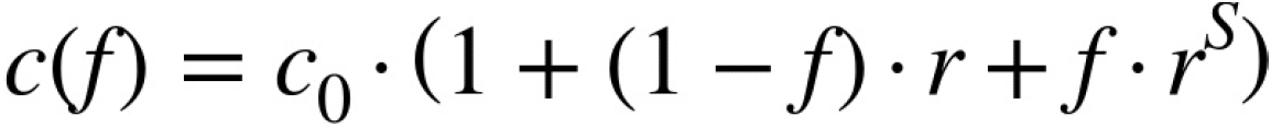
c(f) = c0 + increased capital(base on c0)
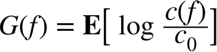
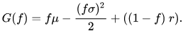
Here, r is the constant short rate earned on cash not invested in the stock. Maximizing the geometric
growth rate means maximizing the term:
Assume now that there are n relevant trading days in the year so that for each such trading day i:
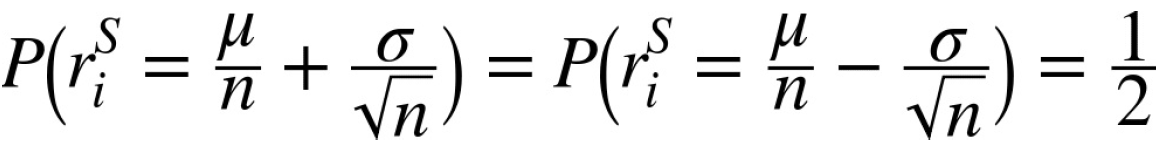
Note that volatility ![]() scales with the square root of the number of trading days. Under these
scales with the square root of the number of trading days. Under these
assumptions, the daily values scale up to the yearly ones from before and one gets:
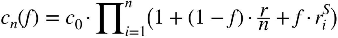
连乘求积
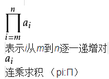
log (![]() ) will convert to
) will convert to ![]()
One now has to maximize the following quantity to achieve maximum long-term wealth when
investing in the stock:

#########################################################
X: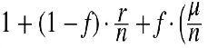
y: ![]()
![]()
(x+y) * (x-y) = x^2 -y^2
#########################################################
Using a Taylor series expansion, one finally arrives at:
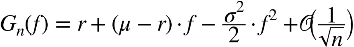
or for infinitely many trading points in time — i.e., for continuous trading — at:
The
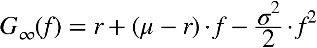
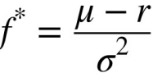
The optimal fraction ![]() then is given through the first-order condition by the expression:
then is given through the first-order condition by the expression:
the first of derivative G(f) = (u-r) * 1 - (std ^2)/2 * 2f =0 then
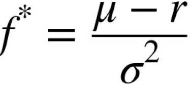
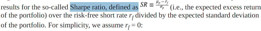
I.e., the expected excess return of the stock over the risk-free rate divided by the variance of the
returns. This expression looks similar to the Sharpe ratio (see “Portfolio Optimization”) but is
different.
##############################################################################
##############################################################################
A real-world example shall illustrate the application of these formulae and their role in leveraging
equity deployed to trading strategies. The trading strategy under consideration is simply a passive被动
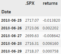
long position in the S&P 500 index. To this end, base data is quickly retrieved and required statistics
are easily derived:
raw = pd.read_csv('../source/tr_eikon_eod_data.csv', index_col=0, parse_dates=True)
symbol = '.SPX'
data = pd.DataFrame( raw[symbol])
data['returns'] = np.log(data/data.shift(1))
data.dropna(inplace=True) #since shift will generate a null in first row
data.tail()
The statistical properties of the S&P 500 index over the period covered suggest an optimal fraction of about 4.5 to be invested in the long position in the index. In other words, for every dollar available 4.5 dollars shall be invested — implying a leverage ratio of 4.5, in accordance with the optimal Kelly “fraction” (or rather “factor” in this case). Ceteris paribus, the Kelly criterion implies a higher leverage the higher the expected return and the lower the volatility (variance):
mu = data.returns.mean() * 252 #Calculates the annualized return.
mu
![]()
sigma = data.returns.std() * 252 ** 0.5 #Calculates the annualized volatility.
sigma
![]()
r =0.0 #Sets the risk-free rate to 0 (for simplicity).
f = (mu-r) / sigma**2 #Calculates the optimal Kelly fraction to be invested in the strategy.
f
![]() # about 4.5 # a leverage ratio of 4.5
# about 4.5 # a leverage ratio of 4.5
The following code simulates the application of the Kelly criterion and the optimal leverage ratio.
For simplicity and comparison reasons, the initial equity is set to 1 while the initially invested total
capital is set to ![]() . Depending on the performance of the capital deployed to the strategy, the total
. Depending on the performance of the capital deployed to the strategy, the total
capital itself is adjusted daily according to the available equity. After a loss, the capital is reduced;
after a profit, the capital is increased. The evolution of the equity position compared to the index
itself is shown in Figure:
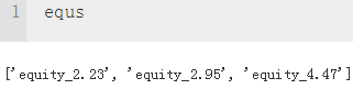
equs =[]
data.head()

def kelly_strategy(f):
global equs
equ = 'equity_{:.2f}'.format(f)
equs.append(equ)
cap = 'capital_{:.2f}'.format(f)
data[equ] =1 #Generates a new column for equity and sets the initial value to 1.
data[cap] = data[equ] * f #Generates a new column for capital and sets the initial value to 1*f.
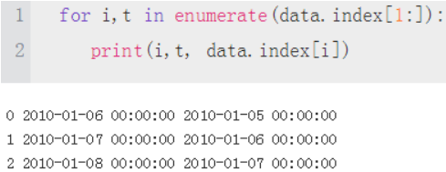
for i,t in enumerate(data.index[1:]): #i,t: index, timestamp
t_1 = data.index[i] #t_1: 2010-01-05 00:00:00 #t: 2010-01-06 00:00:00
#data[cap].loc[t_1]: previous capital(at time t-1)
#Calculates the new capital position(at time t) given the return.
#initial pre_cap = equity*f = 1*f
#current cap(ratio)=pre_cap(ratio) * Return Rate
data.loc[t, cap] = data[cap].loc[t_1] * math.exp(data['returns'].loc[t])
#Adjusts the equity value according to the capital position performance.
#current equity = current cap(ratio) - pre cap(ratio) + pre equity
#profit or loss
data.loc[t, equ] = data[cap].loc[t] - data[cap].loc[t_1] + data[equ].loc[t_1]
#Adjusts the capital position given the new equity position and the fixed leverage ratio.
#adusted current cap = current equ * f
data.loc[t, cap] = data[equ].loc[t] * f
kelly_strategy(f*0.5) #Simulates the Kelly criterion–based strategy for half of f …
kelly_strategy(f*0.66) #… for two-thirds of f …
kelly_strategy(f) #… and for f itself.
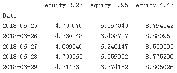
print(data[equs].tail())
colormap={
'returns':'m', #puple-red
'equity_2.23':'b', #blue
'equity_2.95':'y', #yellow
'equity_4.47':'r', #red
}
ax = data['returns'].cumsum().apply(np.exp).plot(legend=True, figsize=(10,6),
style=colormap,
title='Cumulative performance of S&P 500 compared to equity position given different values of f')
#ax=ax at the same plotting
data[equs].plot(ax=ax, legend=True,style=colormap)

As Figure illustrates, applying the optimal Kelly leverage leads to a rather erratic evolution不稳定的演变of the equity position (high volatility) which is — given the leverage ratio of 4.47 — intuitively plausible. One would expect the volatility of the equity position to increase with increasing leverage(ratio). Therefore, practitioners often reduce the leverage to, for example, “half Kelly” — i.e., in the current example to . Therefore, Figure 16-3 also shows the evolution of the equity position of values lower than “full Kelly.” The risk indeed reduces with lower values of f.
ML-Based Trading Strategy
Chapter 14 introduces the FXCM trading platform, its REST API, and the Python wrapper package
fxcmpy. This section combines an ML-based approach for predicting the direction of market price
movements with historical data from the FXCM REST API to backtest an algorithmic trading strategy
for the EUR/USD currency pair. It uses vectorized backtesting, taking into account this time the bid-ask
spread as proportional transaction costs. It also adds, compared to the plain vectorized backtesting
approach as introduced in Chapter 15, a more in-depth analysis of the risk characteristics of the
trading strategy tested.
https://www.fxcm.com/uk/forex-trading-demo/
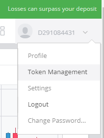
Login: D291084431
Password: 9398

Click "LAUNCH WEB PLATFORM"

Password: 9398
on the top right, click your account then click "Token Management"
Password: 9398

Next:

Click Copy button: 5f20afae941cd6bc981f3f850c991885b3dae125
Then create a fxcm.cfg file

###############################################
bid price是买家愿意支付的最高价格,还有很多价格,不过都低于这个最高价位。
ask price是卖家出的最低价格,还有其他报价,但都高于这个价格。
BID是买入价
ASK是卖出价
在外汇里买入叫做多,卖出叫做空。做多就是你买了一笔交易然后等价钱涨上去再卖这样你就赢利了,卖空就是你付了保证金后公司借给你这些保证金的货币,然后等价格跌下去了你再把这些货币还给公司。
ask price 或者offer price 要价 卖方报价
任何潜在出售者能够接受的最低价格
bid price 出价 买方报价
任何潜在的购买者愿意支付的最高价格
ask是卖出价;bid是买入价
###############################################
#https://www.fxcm.com/fxcmpy/00_quick_start.html
#https://blog.csdn.net/Linli522362242/article/details/102816913
import fxcmpy
fxcmpy.__version__
![]()
#Connects to the API and retrieves the data.
api = fxcmpy.fxcmpy(config_file='fxcm.cfg')
# OR api = fxcmpy.fxcmpy(access_token='5f20afae941cd6bc981f3f850c991885b3dae125', log_level='error')
data = api.get_candles('EUR/USD', period='m5', start='2018-06-01 00:00:00', stop='2018-06-30 00:00:00')
data.iloc[-5:, 4:]

data.info()

#Calculates the average bid-ask spread.
spread = (data['askclose']-data['bidclose']).mean()
spread
![]()
#Calculates the mid close prices from the ask and bid close prices.
data['midclose'] = (data['askclose'] + data['bidclose']) /2
ptc = spread / data['midclose'].mean()
ptc
![]()
data['midclose'].plot(figsize=(10,6), legend=True, title='EUR/USD exchange rate (five-minute bars)')

The ML-based strategy is based on lagged return data that is binarized. In other words, the ML algorithm learns from historical patterns of upward and downward movements whether another upward or downward movement is more likely. Accordingly, the following code creates features data with values of 0 and 1 as well as labels data with values of +1 and -1 indicating the observed market direction in all cases:
data['returns'] = np.log(data['midclose'] / data['midclose'].shift(1))
data.dropna(inplace=True) #since shift
lags=5
cols = []
for lag in range(1, lags+1):
col = 'lag_{}'.format(lag)
#Creates the lagged return data given the number of lags.
data[col] = data['returns'].shift(lag)
cols.append(col)
data.head()

cols
![]()
Accordingly, the following code creates features data with values of 0 and 1 as well as labels data with values of +1 and -1 indicating the observed market direction in all cases:
The basic idea behind the usage of lagged log returns as features is that they might be informative in predicting future returns. For example, one might hypothesize that after two downward movements an upward movement is more likely (“mean reversion”), or, to the contrary, that another downward movement is more likely (“momentum” or “trend”). The application of regression techniques allows the formalization of such informal reasonings.
data.dropna(inplace=True) #since shift
#Transforms the feature values to binary data.
data[cols] = np.where(data[cols]>0, 1, 0)
#Transforms the returns data to directional label data.
data['direction'] = np.where(data['returns']>0, 1,-1)
data[cols+['direction']].head()

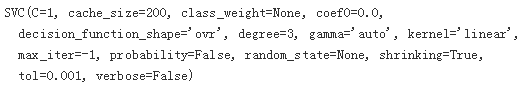
from sklearn.svm import SVC
from sklearn.metrics import accuracy_score
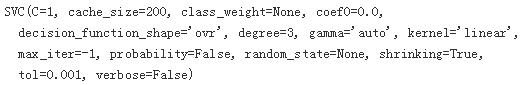
model = SVC(C=1, kernel='linear', gamma='auto')
split = int(len(data)*0.8)
train = data.iloc[:split].copy()
model.fit(train[cols], train['direction'])
#The accuracy of the predictions from the trained model in-sample (training data).
accuracy_score(train['direction'], model.predict(train[cols]))
![]()
test = data.iloc[split:].copy()
test['position'] = model.predict(test[cols])
#The accuracy of the predictions from the trained model out-of-sample (test data).
accuracy_score(test['direction'], test['position'])
![]()
It is well known that the hit ratio is only one aspect of success in financial trading. Also crucial are, among other things, the transaction costs implied by the trading strategy and getting the important trades right. To this end, only a formal vectorized backtesting approach allows judgment of the quality of the trading strategy. The following code takes into account the proportional transaction costs based on the average bid-ask spread. Figure compares the performance of the algorithmic trading strategy (without and with proportional transaction costs) to the performance of the passive benchmark investment:
test.head()

#Derives the log returns for the ML-based algorithmic trading strategy.
test['strategy'] = test['position'] * test['returns']
#######################################################
DataFrame.diff(self, periods=1, axis=0) First discrete difference of element.
Calculates the difference of a DataFrame element compared with another element in the DataFrame (default is the element in the same column of the previous row).

#######################################################
#Calculates the number of trades implied by the trading strategy based on changes in the position.
sum(test['position'].diff() !=0) #axis=0
![]()
#Whenever a trade takes place, the proportional transaction costs(ptc) are subtracted from the
#strategy’s log return on that day.
#data['returns'] = np.log(data['midclose'] / data['midclose'].shift(1))
test['strategy_tc'] = np.where(test['position'].diff() !=0,
test['strategy']-ptc *0.15, #Originally, the ptc=ptc*1.0
test['strategy'])
test.head()

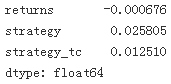
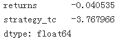
test[['returns', 'strategy', 'strategy_tc']].sum()
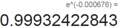
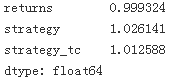
test[['returns', 'strategy', 'strategy_tc']].sum().apply(np.exp)
test[['returns', 'strategy','strategy_tc']].cumsum().apply(np.exp).plot(figsize=(10,6),
title='Performance of EUR/USD exchange rate and algorithmic trading strategy')


############################################################################
VS the author's figure Note: returns and strategy_tc since the author's ptc=0.15*ptc

############################################################################
LIMITATIONS OF VECTORIZED BACKTESTING
Vectorized backtesting has its limits with regard to how closely to market realities strategies can be tested. For example, it does not allow direct inclusion of fixed transaction costs per trade. One could, as an approximation, take a multiple of the average proportional transaction costs (based on average position sizes) to account indirectly for fixed transactions costs. However, this would not be precise in general. If a higher degree of precision is required other approaches, such as eventbased backtesting with explicit loops over every bar of the price data, need to be applied.
Optimal Leverage
Equipped with the trading strategy’s log returns data, the mean and variance values can be calculated in order to derive the optimal leverage according to the Kelly criterion. The code that follows scales the numbers to annualized values, although this does not change the optimal leverage values according to the Kelly criterion since the mean return and the variance scale with the same factor:
#Annualized mean returns.
#Connects to the API and retrieves the data.
#data = api.get_candles('EUR/USD',
# period='m5', #every 5 minutes
# start='2018-06-01 00:00:00',
# stop='2018-06-30 00:00:00'
# )
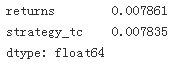
mean = test[['returns', 'strategy_tc']].mean() * len(data) * 12 #12 months
mean
#Annualized variances.
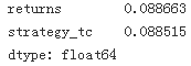
var = test[['returns', 'strategy_tc']].var() * len(data) * 12
var
#Annualized volatilities
vol = var **0.5
vol
#Optimal leverage according to the Kelly criterion (“full Kelly”).
mean / var # fraction f = (mu - r) / sigma ** 2 since we set r=0
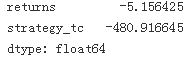
Using the “half Kelly” criterion, the optimal leverage for the trading strategy is about 40. With a number of brokers, such as FXCM, and financial instruments, such as foreign exchange and contracts for difference (CFDs), such leverage ratios are feasible, even for retail traders. Figure shows in comparison the performance of the trading strategy with transaction costs for different leverage values:
to_plot = ['returns', 'strategy_tc']
for lev in [10,20,30,40,50]:
label = 'lstrategy_tc_%d' % lev
test[label] = test['strategy_tc'] * lev #Scales the strategy returns for different leverage values.
to_plot.append(label)

test[to_plot].cumsum().apply(np.exp).plot(figsize=(10,6),
title='Performance of algorithmic trading strategy for different leverage values'
)

Risk Analysis
Since leverage increases the risk associated with a trading strategy, a more in-depth risk analysis seems in order. The risk analysis that follows assumes a leverage ratio of 30. First, the maximum drawdown缩水 and the longest drawdown period are calculated. Maximum drawdown最大跌幅 is the largest loss (dip) after a recent high. Accordingly, the longest drawdown period最长的回撤期 is the longest period that the trading strategy needs to get back to a recent high. The analysis assumes that the initial equity position is 3,333 EUR, leading to an initial position size of 100,000 EUR for a leverage ratio of 30(100,000/30=3,333 EUR). It also assumes that there are no adjustments with regard to the equity over time, no matter what the performance is(profit/loss from capital):
#The initial equity.
equity = 3333
#The relevant log returns time series
risk = pd.DataFrame(test['lstrategy_tc_30'])
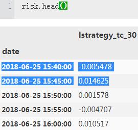
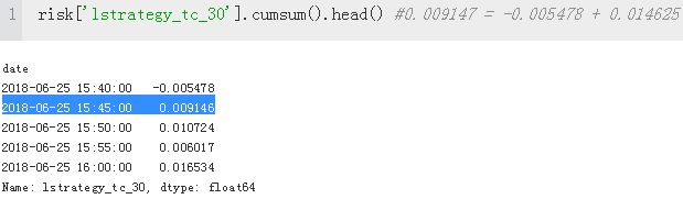
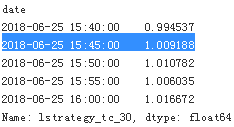
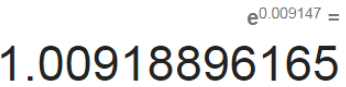
risk['lstrategy_tc_30'].cumsum().apply(np.exp).head()
#… scaled by the initial equity.
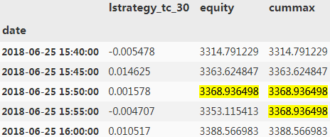
risk['equity'] = risk['lstrategy_tc_30'].cumsum().apply(np.exp) * equity

#The cumulative maximum values over time.
risk['cummax'] = risk['equity'].cummax()
risk.head()
#The drawdown values over time.
#Maximum drawdown最大跌幅 is the largest loss (dip) after a recent high.
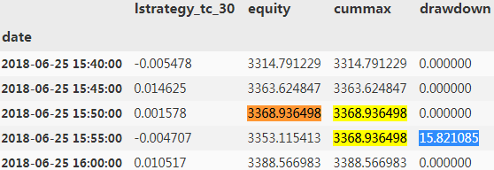
risk['drawdown'] = risk['cummax'] - risk['equity']
risk.head()
#The maximum drawdown value.
risk['drawdown'].max()
![]()
#The point in time when it happens.
t_max = risk['drawdown'].idxmax()
t_max
![]()
Technically a (new) high is characterized by a drawdown value of 0(for instances,3314.791229: 0.000000, 3363.624847:0.000000, and so on). The drawdown period is the time between two such highs. Figure visualizes both the maximum drawdown and the drawdown periods:
#Identifies highs for which the drawdown must be 0
temp = risk['drawdown'][risk['drawdown']==0]
temp.head()
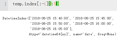
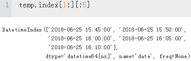
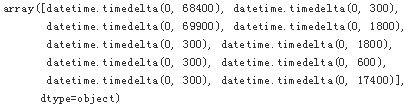
#The drawdown period is the time between two such highs.
#Calculates the timedelta values between all highs.
periods = (temp.index[1:].to_pydatetime() - temp.index[:-1].to_pydatetime())
periods[20:30]
#the longest drawdown period最长的回撤期 is the longest period that the trading strategy needs to get back to a recent high.
#The longest drawdown period in seconds …
t_per = periods.max()
t_per
![]()
#… and hours.
t_per.seconds / 60 /60
![]()
#The cumulative maximum values over time. #risk['cummax'] = risk['equity'].cummax()
risk[['equity', 'cummax']].plot(figsize=(10,6),
title='Maximum drawdown (vertical line) and drawdown periods (horizontal lines)'
)
#t_max = risk['drawdown'].idxmax() #The point in time when it happens.
plt.axvline(t_max, c='k', alpha=0.5) #alpha: transparence #The maximum drawdown value.

https://blog.csdn.net/Linli522362242/article/details/96593981
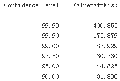
Another important risk measure is value-at-risk (VaR). It is quoted as a currency amount and represents the maximum loss to be expected given both a certain time时间范围 horizon and a confidence level. The code that follows derives VaR values based on the log returns of the equity position for the leveraged trading strategy over time for different confidence levels. The time interval is fixed to the bar length of five minutes:
import scipy.stats as scs
#Defines the percentile values to be used.
percs = np.array([0.01, 0.1, 1., 2.5, 5.0, 10.0])
risk['returns'] = np.log(risk['equity'] / risk['equity'].shift(1))

VaR = scs.scoreatpercentile(equity * risk['returns'], percs)

def print_var():
print('%16s %16s' % ('Confidence Level', 'Value-at-Risk'))
print(33*'-')
for pair in zip(percs, VaR):
#Translates the percentile values into confidence levels and the VaR values (negative values) to
#positive values for printing.
print('%16.2f %16.3f' % (100-pair[0], -pair[1])) #percs = np.array([0.01, 0.1, 1., 2.5, 5.0, 10.0])
print_var()
##############################################
Having the ndarray object with the sorted results, the function scoreatpercentile already does the trick. All we have to do is to define the percentiles (in percent values) in which we are interested. In the list object percs, 0.1 translates into a confidence level of 100% – 0.1% = 99.9%. The 30-day VaR given a confidence level of 99.9% in this case is 175.879 currency units, while it is 31.896 at the 90% confidence level
##############################################
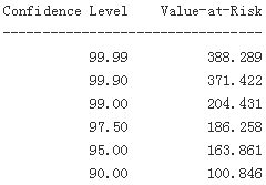
Finally, the following code calculates the VaR values for a time horizon of one hour by resampling the original DataFrame object. In effect, the VaR values are increased for all confidence levels but the highest one:


#Resamples the data from five-minute to one-hour bars.
hourly = risk.resample('1H', label='right').last() #1H : a sample frequency
hourly['returns'] = np.log(hourly['equity'] / hourly['equity'].shift(1))
VaR = scs.scoreatpercentile(equity * hourly['returns'], percs)
print_var() #for one hour by resampling #the VaR values are increased for all confidence levels but the highest one:
Persisting the Model Object
Once the algorithmic trading strategy is “accepted” based on the backtesting, leveraging, and risk analysis results, the model object might be persisted for later use in deployment. It embodies now the ML-based trading strategy or the trading algorithm:
import pickle
pickle.dump(model, open('algorithm.pkl', 'wb'))
![]()
Online Algorithm
The trading algorithm tested so far is an offline algorithm. Such algorithms use a complete data set to solve a problem at hand. The problem has been to train an SVM algorithm based on binarized features data and directional label data. In practice, when deploying the trading algorithm in financial markets, it must consume data piece-by-piece as it arrives to predict the direction of the market movement for the next time interval (bar). This section makes use of the persisted model object from the previous section and embeds it into a streaming data environment.
The code that transforms the offline trading algorithm into an online trading algorithm mainly addresses the following issues:
Tick data Tick data arrives in real time and is to be processed in real time
Resampling The tick data is to be resampled to the appropriate bar size given the trading algorithm
Prediction The trading algorithm generates a prediction for the direction of the market movement over the relevant time interval that by nature lies in the future
Orders Given the current position and the prediction (“signal”) generated by the algorithm, an order is placed or the position is kept
“Retrieving Streaming Data” shows how to retrieve tick data from the FXCM REST API in real time. The basic approach is to subscribe to a market data stream and pass a callback function that processes the data.
First, the persisted trading algorithm is loaded — it represents the trading logic to be followed. It might also be useful to define a helper function to print out the open position(s) while the trading algorithm is trading:
algorithm = pickle.load(open('algorithm.pkl', 'rb'))
algorithm
#Defines the DataFrame columns to be shown.
sel = ['tradeId', 'amountK', 'currency', 'grossPL', 'isBuy']
def print_positions(pos):
print( '\n\n' + 50*'=' )
print( 'Going {}.\n'.format(pos))
#Waits a bit for the order to be executed and reflected in the open positions
time.sleep(1.5)
#Prints the open positions.
print(api.get_open_positions()[sell])
print( 50*'=' + '\n\n')
Before the online algorithm is defined and started, a few parameter values are set:

#Instrument symbol to be traded.
symbol ='EUR/USD'
#Bar length for resampling; for easier testing, the bar length might be shortened compared to the
#real deployment length (e.g., 15 seconds instead of 5 minutes).
bar = '15s'
#The amount, in thousands, to be traded.
amount = 100
#The initial position (“neutral”).
position=0
#The minimum number of resampled bars required for the first prediction and trade to be
#possible.
min_bars = lags+1
#An empty DataFrame object to be used later for the resampled data.
df = pd.DataFrame()
Following is the callback function automated_strategy() that transforms the trading algorithm into a real-time context:
##############################################################
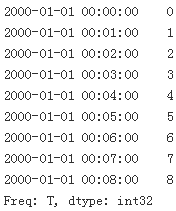
index = pd.date_range('1/1/2000', periods=9, freq='T') #T : minute
series = pd.Series(range(9), index=index)
series
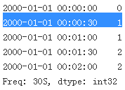
series.resample('30S')[0:5]

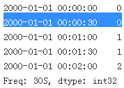
series.resample('30S').bfill()[0:5]
series.resample('30S').ffill()[0:5]
##############################################################
def automated_strategy(data, dataframe):
global min_bars, position, df
ldf = len(dataframe) #Captures the length of the DataFrame object with the tick data.
#Resamples the tick data to the defined bar length.
df = dataframe.resample(bar, label='right').last().ffill()
if ldf % 20==0:
print('%3d' % len(dataframe), end=',')
if len(df) > min_bars:
min_bars = len(df)
df['Mid'] = df[['Bid', 'Ask']].mean(axis=1)
df['Returns'] = np.log( df['Mid'] / df['Mid'].shift(1) )
df['Direction'] = np.where(df['Returns'] >0, 1, -1)
features = df['Direction'].iloc[-(lags+1):-1] #Picks the relevant feature values for all lags …
#… and reshapes them to a form that the model can use for prediction
features = features.values.reshape(1,-1) #one row, columns will be automally adjusted
signal = algorithm.predict(features)[0] #Generates the prediction value (either +1 or -1).
#The conditions to enter (or keep) a long position.
##The initial position (“neutral”). #position=0
#current position==-1
if position in [0,-1] and signal==1:
api.create_market_buy_order(
symbol, amount -position *amount
)
position =1
print_positions['LONG']
#The conditions to enter (or keep) a short position.
#current position==1
elif position in [0,1] and signal==-1:
api.create_market_sell_order(
symbol, amount +position * amount
)
position =-1
print_positions['SHORT']
#The condition to stop trading and close out any open positions (arbitrarily defined based on the
#number of ticks retrieved).
if len(dataframe) > 350:#
api.unsubscribe_market_data('EUR/USD')
api.close_all()
Infrastructure and Deployment
Deploying an automated algorithmic trading strategy with real funds requires an appropriate
infrastructure. Among others, the infrastructure should satisfy the following conditions:
Reliability
The infrastructure on which to deploy an algorithmic trading strategy should allow for high
availability (e.g., > 99.9%) and should otherwise take care of reliability (automatic backups,
redundancy of drives and web connections, etc.).
Performance
Depending on the amount of data being processed and the computational demand the algorithms
generate, the infrastructure must have enough CPU cores, working memory (RAM), and storage
(SSD); in addition, the web connections should be sufficiently fast.
Security
The operating system and the applications run on it should be protected by strong passwords as
well as SSL encryption; the hardware should be protected from fire, water, and unauthorized
physical access.
Basically, these requirements can only be fulfilled by renting appropriate infrastructure from a
professional data center or a cloud provider. Investments in the physical infrastructure to satisfy the
aforementioned前述的 requirements can in general only be justified by the bigger or even biggest players in
the financial markets
From a development and testing point of view, even the smallest Droplet (cloud instance) from
DigitalOcean is enough to get started. At the time of this writing such a Droplet costs 5 USD per
month; usage is billed by the hour and a server can be created within minutes and destroyed within
seconds.
How to set up a Droplet with DigitalOcean is explained in detail in the section “Using Cloud
Instances”, with bash scripts that can be adjusted to reflect individual requirements regarding Python
packages, for example.
OPERATIONAL RISKS
Although the development and testing of automated algorithmic trading strategies is possible from a local computer
(desktop, notebook, etc.), it is not appropriate for the deployment of live strategies trading real money. A simple loss of the
web connection or a brief power outage might bring down the whole algorithm算法瘫痪, leaving, for example, unintended open positions in the portfolio or causing data set corruption (due to missing out on real-time tick data), potentially leading to wrong signals and unintended trades/positions.
Logging and Monitoring
Let’s assume that the automated algorithmic trading strategy is to be deployed on a remote server
(cloud instance, leased server, etc.), that all required Python packages have been installed (see
“Using Cloud Instances”), and that, for instance, Jupyter Notebook is running securely. What else
needs to be considered from the algorithmic trader’s point of view if they do not want to sit all day in
front of the screen while logged in to the server?
This section addresses two important topics in this regard: logging and real-time monitoring.
Logging persists information and events on disk for later inspection. It is standard practice in
software application development and deployment. However, here the focus might be put rather on
the financial side, logging important financial data and event information for later inspection and
analysis. The same holds true for real-time monitoring making use of socket communication. Via
sockets a constant real-time stream of important financial aspects can be created that can be retrieved
and processed on a local computer, even if the deployment happens in the cloud.
“Automated Trading Strategy” presents a Python script implementing all these aspects and making use
of the code from “Online Algorithm”. The script puts the code in a shape that allows, for example, the
deployment of the algorithmic trading strategy — based on the persisted algorithm object — on a
remote server. It adds both logging and monitoring capabilities based on a custom function that,
among others, makes use of ZeroMQ for socket communication. In combination with the short script
from “Strategy Monitoring”, this allows for remote real-time monitoring of the activity on a remote
server.
When the script from “Automated Trading Strategy” is run, either locally or remotely, the output that
is logged and sent via the socket looks as follows:


my run:

Running the script from “Strategy Monitoring” locally then allows the real-time retrieval and
processing of such information. Of course, it is easy to adjust the logging and streaming data to one’s
own requirements. Similarly, one can also, for example, persist DataFrame objects as created during
the execution of the trading script. Furthermore, the trading script and the whole logic can be adjusted
to include such elements as stop losses or take profit targets programmatically. Alternatively, one
could make use of more sophisticated order types available via the FXCM trading API
CONSIDER ALL RISKS
Trading currency pairs and/or CFDs is associated with a number of financial risks. Implementing an algorithmic trading
strategy for such instruments automatically leads to a number of additional risks. Among them are flaws in the trading
and/or execution logic. as well as technical risks such as problems with socket communications or delayed retrieval or even
loss of tick data during the deployment. Therefore, before one deploys a trading strategy in automated fashion one should
make sure that all associated market, execution, operational, technical, and other risks have been identified, evaluated, and
addressed. The code presented in this chapter is intended only for technical illustration purposes.
Conclusion
This chapter is about the deployment of an algorithmic trading strategy — based on a classification
algorithm from machine learning to predict the direction of market movements — in automated
fashion. It addresses such important topics as capital management (based on the Kelly criterion),
vectorized backtesting for performance and risk, the transformation of offline to online trading
algorithms, an appropriate infrastructure for deployment, as well as logging and monitoring during
deployment.
The topic of this chapter is complex and requires a broad skill set from the algorithmic trading
practitioner. On the other hand, having a REST API for algorithmic trading available, such as the one
from FXCM, simplifies the automation task considerably since the core part boils down mainly to
making use of the capabilities of the Python wrapper package fxcmpy for tick data retrieval and order
placement. Around this core, elements to mitigate operational and technical risks as far as possible
have to be added.
Automated Trading Strategy
The following is the Python script to implement the algorithmic trading strategy in automated fashion,
including logging and monitoring.
!cat automated_strategy.py
import zmq
import time
import pickle
import fxcmpy
import numpy as np
import pandas as pd
import datetime as dt

sel = ['tradeId', 'amountK', 'currency',
       'grossPL', 'isBuy']

log_file = 'automated_strategy.log'

# loads the persisted algorithm object
algorithm = pickle.load(open('algorithm.pkl', 'rb'))

# sets up the socket communication via ZeroMQ (here: "publisher")
context = zmq.Context()
socket = context.socket(zmq.PUB)

# this binds the socket communication to all IP addresses of the machine
socket.bind('tcp://0.0.0.0:5555')


def logger_monitor(message, time=True, sep=True):
    ''' Custom logger and monitor function.
    '''
    with open(log_file, 'a') as f:
        t = str(dt.datetime.now())
        msg = ''
        if time:
            msg += '\n' + t + '\n'
        if sep:
            msg += 66 * '=' + '\n'
        msg += message + '\n\n'
        # sends the message via the socket
        socket.send_string(msg)
        # writes the message to the log file
        f.write(msg)


def report_positions(pos):
    ''' Prints, logs and sends position data.
    '''
    out = '\n\n' + 50 * '=' + '\n'
    out += 'Going {}.\n'.format(pos) + '\n'
    time.sleep(2)  # waits for the order to be executed
    out += str(api.get_open_positions()[sel]) + '\n'
    out += 50 * '=' + '\n'
    logger_monitor(out)
    print(out)


def automated_strategy(data, dataframe):
    ''' Callback function embodying the trading logic.
    '''
    global min_bars, position, df
    # resampling of the tick data
    df = dataframe.resample(bar, label='right').last().ffill()

    if len(df) > min_bars:
        min_bars = len(df)
        logger_monitor('NUMBER OF BARS: ' + str(min_bars))
        # data processing and feature preparation
        df['Mid'] = df[['Bid', 'Ask']].mean(axis=1)
        df['Returns'] = np.log(df['Mid'] / df['Mid'].shift(1))
        df['Direction'] = np.where(df['Returns'] > 0, 1, -1)
        # picks relevant points
        features = df['Direction'].iloc[-(lags + 1):-1]
        # necessary reshaping
        features = features.values.reshape(1, -1)
        # generates the signal (+1 or -1)
        signal = algorithm.predict(features)[0]

        # logs and sends major financial information
        logger_monitor('MOST RECENT DATA\n' +
                       str(df[['Mid', 'Returns', 'Direction']].tail()),
                       False)
        logger_monitor('features: ' + str(features) + '\n' +
                       'position: ' + str(position) + '\n' +
                       'signal:   ' + str(signal), False)

        # trading logic
        if position in [0, -1] and signal == 1:  # going long?
            api.create_market_buy_order(
                symbol, size - position * size)  # places a buy order
            position = 1  # changes position to long
            report_positions('LONG')

        elif position in [0, 1] and signal == -1:  # going short?
            api.create_market_sell_order(
                symbol, size + position * size)  # places a sell order
            position = -1  # changes position to short
            report_positions('SHORT')
        else:  # no trade
            logger_monitor('no trade placed')

        logger_monitor('****END OF CYCLE***\n\n', False, False)

    if len(dataframe) > 350:  # stopping condition
        api.unsubscribe_market_data('EUR/USD')  # unsubscribes from data stream
        report_positions('CLOSE OUT')
        api.close_all()  # closes all open positions
        logger_monitor('***CLOSING OUT ALL POSITIONS***')


if __name__ == '__main__':
    symbol = 'EUR/USD'  # symbol to be traded
    bar = '15s'  # bar length; adjust for testing and deployment
    size = 100  # position size in thousand currency units
    position = 0  # initial position
    lags = 5  # number of lags for features data
    min_bars = lags + 1  # minimum length for resampled DataFrame
    df = pd.DataFrame()
    # adjust configuration file location
    api = fxcmpy.fxcmpy(config_file='../fxcm.cfg')
    # the main asynchronous loop using the callback function
    api.subscribe_market_data(symbol, (automated_strategy,))
!cat strategy_monitoring.py

import zmq

# sets up the socket communication via ZeroMQ (here: "subscriber")
context = zmq.Context()
socket = context.socket(zmq.SUB)

# adjust the IP address to reflect the remote location if necessary
socket.connect('tcp://206.189.51.42:5555')

# configures the socket to retrieve every message
socket.setsockopt_string(zmq.SUBSCRIBE, '')

while True:
    msg = socket.recv_string()
    print(msg)
