1.介绍
2017年IEE IGRASS多光谱影像分类比赛,选用两个卫星landsat_8和sentinel_2所拍摄的多光谱图像作为输入,输出像素级分类图像。其中landsat_8有4个时段的影像数据,sentinel_2只有一个时段的影像数据。拍摄城市有巴黎/柏林/罗马/香港/圣保罗 五个地区,模型选用前4个地区的数据作为训练样本,圣保罗地区数据作为测试样本。依次选取landsat_8的每个时段数据与sentinel_2的数据组合,作为输入数据,输出为所属种类。开始采用分割图的方法,将训练影像分割为若干个28*28*channel 的小图,每个小图的label对应为中心像素点坐标在groundtruth上划分的种类。训练模型选用双通道2层CNN架构,即(conv+relu+pool)*2,最后一层将双通道的稀疏特征进行级联,作为最终的特征向量,再通过2层全连接层,并送入softmax层输出最终分类结果。训练时采用dropout和全连接层权值正则化的方式防止过拟合,在训练样本的采集方面也先进行了边缘填充,并将各个种类的样本都选择1000个,不够1000的则全部选用,以保证样本的多样性和平衡性,并对数据进行归一化。在最后的测试时,将landsat_8的4个时段的预测结果进行投票打分,最后选择得分最高的类作为最终label。在对数据进行划分时,可以采用稀疏采样,用5*5像素块对原始图进行滑窗操作,若块内像素类全部相同且不是背景类,则间隔一个像素进行稀疏采样,只选取一半的像素点作为训练数据,以保证训练样本的多样性,最后测试结果显示,稀疏采样可提高模型预测的准确率。
2.代码:
# This Python file uses the following encoding: utf-8

import tensorflow as tf           # 深度学习框架
import matplotlib.pyplot as plt   # 画图包
import numpy as np                # 矩阵运算包
import scipy.io                   # 保存图片
from PIL import Image             # 图像处理
from tqdm import tqdm             # 进度条
import os                         # 读取文件
import time                       # 获取时钟时间
import h5py                       # 读取文件
import sys                        # 系统输出格式


# 定义输入图像的大小 28*28
IMAGE_SIZE = 28

# 两个卫星的通道数,分别为9和10
NUM_CHANNELS_1 = 9
NUM_CHANNELS_2 = 10

# 像素值0~255
PIXEL_DEPTH = 255

# 分类个数为17
NUM_LABELS = 17

# 验证集共有1000个样本
VALIDATION_SIZE = 1000

# 设置随机种子大小
# SEED = np.random.randint(1, 10**5)
SEED = 52014

# 批量处理BATCH大小
BATCH_SIZE = 30

# 训练代数
NUM_EPOCHS = 50

# 验证集批量处理大小
EVAL_BATCH_SIZE = 256

# 验证时间间隔,每训练多少个批次做一次评估
EVAL_FREQUENCY = 5000

tf.app.flags.DEFINE_boolean("self_test", False, "True if running a self test.")
FLAGS = tf.app.flags.FLAGS


# 假数据,用于功能检测
def fake_data(num_images):
    data1 = np.ndarray(
        shape=(num_images, IMAGE_SIZE, IMAGE_SIZE, NUM_CHANNELS_1),
        dtype=np.int32)
    data2 = np.ndarray(
        shape=(num_images, IMAGE_SIZE, IMAGE_SIZE, NUM_CHANNELS_2),
        dtype=np.int32)
    labels = np.zeros(shape=(num_images,), dtype=np.int32)

    data1 = np.random.randint(0, 255, size=data1.shape)
    data2 = np.random.randint(0, 255, size=data2.shape)
    labels = np.random.randint(0, NUM_LABELS-1, size=labels.shape)
    return data1, data2, labels

# 计算匪类错误率
def error_rate(predictions, labels):
    correction = np.sum(np.argmax(predictions, axis=1) == labels) / predictions.shape[0]
    return (1 - correction) * 100


# def main(argv = None):
# matfn = './p_cf_ave_28_city_10928_sparse.mat'
matfn = './learnCNN9428.mat'
# matfn = './learnCNN_sparse9428.mat'

model_path = "./checkpoints-non/model_conMy.ckpt"
# model_path = "./checkpoints-sparse/model_conMy.ckpt"

data = h5py.File(matfn)
arrays = {}
# print(list(data.items()))
for k, v in data.items():
    arrays[k] = np.array(v)

train_data1 = arrays['train_x1']  # 一号卫星输入图片,大小为(10928, 28, 28, 9) 注意:python读入时维度与matlab读入的维度顺序有所不同
# train_data1 = train_data1.transpose(3, 1, 2, 0) # 必要时,可将维度转换成python对应顺序
train_data2 = arrays['train_x2']  # 二号卫星输入图片,大小为(10928, 28, 28, 10)
train_labels = arrays['train_y']  # 图片分类标签,大小为(1, 10928)

train_labels = train_labels.reshape(train_labels.shape[1]).astype(np.int64)  # 将label维度转换为(10928, )
train_labels -= 1  # 类别由从1计数变为从0计数

test_data1 = arrays['yanzheng_x1']
test_data2 = arrays['yanzheng_x2']
test_labels = arrays['yanzheng_y']
test_labels = test_labels.reshape(test_labels.shape[1]).astype(np.int64)
test_labels -= 1  # 类别由从1计数变为从0计数

train_data1 = train_data1.astype(np.float32)
train_data2 = train_data2.astype(np.float32)
test_data1 = test_data1.astype(np.float32)
test_data2 = test_data2.astype(np.float32)

# train_data1 = train_data1 / PIXEL_DEPTH - 0.5  # 将像素值归一化到[-0.5, 0.5]
# train_data2 = train_data2 / PIXEL_DEPTH - 0.5
# test_data1 = test_data1 / PIXEL_DEPTH - 0.5
# test_data2 = test_data2 / PIXEL_DEPTH - 0.5

# 打乱数据
# np.random.seed(SEED)
index = [i for i in range(len(train_data1))]
np.random.shuffle(index)
train_data1 = train_data1[index]
train_data2 = train_data2[index]
train_labels = train_labels[index]

index2 = [i for i in range(len(test_data1))]  # len(array)取的是array数组第一维度的值
np.random.shuffle(index2)
test_data1 = test_data1[index2]
test_data2 = test_data2[index2]
test_labels = test_labels[index2]

# 产生评测集
validation_data1 = test_data1[:VALIDATION_SIZE, ...]
validation_data2 = test_data2[:VALIDATION_SIZE, ...]
validation_labels = test_labels[:VALIDATION_SIZE, ...]

train_size = train_labels.shape[0]

# 训练样本和标签从这里送入网络
train_data_node1 = tf.placeholder(tf.float32, shape=(BATCH_SIZE, IMAGE_SIZE, IMAGE_SIZE, NUM_CHANNELS_1))
train_data_node2 = tf.placeholder(tf.float32, shape=(BATCH_SIZE, IMAGE_SIZE, IMAGE_SIZE, NUM_CHANNELS_2))
train_labels_node = tf.placeholder(tf.int64, shape=(BATCH_SIZE, ))

# 评测数据节点
eval_data_node1 = tf.placeholder(tf.float32, shape=(EVAL_BATCH_SIZE, IMAGE_SIZE, IMAGE_SIZE, NUM_CHANNELS_1))
eval_data_node2 = tf.placeholder(tf.float32, shape=(EVAL_BATCH_SIZE, IMAGE_SIZE, IMAGE_SIZE, NUM_CHANNELS_2))

# 下面的变量为网络的可训练权值,1号卫星
# conv1 权值维度为 5*5*channel1*32, 32为输出特征图数目
conv11_weights = tf.Variable(
    tf.truncated_normal([5, 5, NUM_CHANNELS_1, 32],  # 5*5 filter, depth=32
                        stddev=0.1,
                        seed=SEED),
    name='conv11_weights'
)
# conv1 偏置
conv11_bias = tf.Variable(tf.zeros([32]), name='conv11_bias')

# conv2 权值维度为 5*5*32*64
conv12_weights = tf.Variable(
    tf.truncated_normal([5, 5, 32, 64],
                        stddev=0.1,
                        seed=SEED),
    name='conv12_weights'
)
conv12_bias = tf.Variable(tf.constant(0.1, shape=[64]), name='conv12_bias')

# 下面的变量为网络的可训练权值,2号卫星
# conv1 权值维度为 5*5*channel2*32, 32为输出特征图数目
conv21_weights = tf.Variable(
    tf.truncated_normal([5, 5, NUM_CHANNELS_2, 32],  # 5*5 filter, depth=32
                        stddev=0.1,
                        seed=SEED),
    name='conv21_weights'
)
# conv1 偏置
conv21_bias = tf.Variable(tf.zeros([32]), name='conv21_bias')

# conv2 权值维度为 5*5*32*64
conv22_weights = tf.Variable(
    tf.truncated_normal([5, 5, 32, 64],
                        stddev=0.1,
                        seed=SEED),
    name='conv22_weights'
)
conv22_bias = tf.Variable(tf.constant(0.1, shape=[64]), name='conv22_bias')

# 全连接层 fc1 权值,神经元数目为5122
fc1_weights = tf.Variable(
    tf.truncated_normal([(IMAGE_SIZE // 4) ** 2 * 64 * 2, 512],
                        stddev=0.01,
                        seed=SEED),
    name='fc1_weights'
)
fc1_biases = tf.Variable(tf.constant(0.1, shape=[512]), name='fc1_biases')

fc2_weights = tf.Variable(
    tf.truncated_normal([512, NUM_LABELS],
                        stddev=0.1,
                        seed=SEED),
    name='fc2_weights'
)
fc2_biases = tf.Variable(tf.constant(0.1, shape=[NUM_LABELS]), name='fc2_biases')


# 两个网络并行,双通道CNN,误差共享
# 实现 LeNet-5 模型,该函数输入两组卫星图像数据,输出fc2响应
def model(data1, data2, train=False):
    """the model definition."""
    # 二维卷积,使用“不变形”补零(即输入特征图与输出特征图尺寸一致)
    # 通道一内的卷积运算
    conv1 = tf.nn.conv2d(data1, conv11_weights, strides=[1, 1, 1, 1], padding='SAME')
    # 加偏置,过激活函数一块完成
    relu1 = tf.nn.relu(tf.nn.bias_add(conv1, conv11_bias))
    # 最大值下采样
    pool1 = tf.nn.max_pool(relu1, ksize=[1, 2, 2, 1], strides=[1, 2, 2, 1], padding='SAME')

    # 第二个卷基层
    conv1 = tf.nn.conv2d(pool1, conv12_weights, strides=[1, 1, 1, 1], padding='SAME')
    relu1 = tf.nn.relu(tf.nn.bias_add(conv1, conv12_bias))
    pool1 = tf.nn.max_pool(relu1, ksize=[1, 2, 2, 1], strides=[1, 2, 2, 1], padding='SAME')

    # 特征图变形为2维矩阵,便于送入全连接层
    pool_shape1 = pool1.get_shape().as_list()
    reshape1 = tf.reshape(pool1, [pool_shape1[0], pool_shape1[1] * pool_shape1[2] * pool_shape1[3]])

    # 通道二内的卷积运算
    conv2 = tf.nn.conv2d(data2, conv21_weights, strides=[1, 1, 1, 1], padding='SAME')
    relu2 = tf.nn.relu(tf.nn.bias_add(conv2, conv21_bias))
    pool2 = tf.nn.max_pool(relu2, ksize=[1, 2, 2, 1], strides=[1, 2, 2, 1], padding='SAME')

    conv2 = tf.nn.conv2d(pool2, conv22_weights, strides=[1, 1, 1, 1], padding='SAME')
    relu2 = tf.nn.relu(tf.nn.bias_add(conv2, conv22_bias))
    pool2 = tf.nn.max_pool(relu2, ksize=[1, 2, 2, 1], strides=[1, 2, 2, 1], padding='SAME')

    pool_shape2 = pool2.get_shape().as_list()
    reshape2 = tf.reshape(pool2, [pool_shape2[0], pool_shape2[1] * pool_shape2[2] * pool_shape2[3]])

    # 特征融合
    rs = tf.concat((reshape1, reshape2), 1)

    # 全连接层,注意‘+’运算自动广播偏置
    hidden = tf.nn.relu(tf.matmul(rs, fc1_weights) + fc1_biases)

    # 训练阶段,增加 50% dropout;而测评阶段无需该操作
    if train:
        hidden = tf.nn.dropout(hidden, 0.5, seed=SEED)

    return tf.matmul(hidden, fc2_weights) + fc2_biases    # 最后一步连接softmax层, 因此不需要再进行relu

# 训练阶段计算:对数+交叉熵 损失函数
# 定义网络流图
logits = model(train_data_node1, train_data_node2, True)
loss = tf.reduce_mean(tf.nn.sparse_softmax_cross_entropy_with_logits(logits=logits, labels=train_labels_node)) # labels是一个数,会自动转成one-hot编码

# 全连接层参数进行L2正则化
regularizers = (tf.nn.l2_loss(fc1_weights) + tf.nn.l2_loss(fc1_biases) +
                tf.nn.l2_loss(fc2_weights) + tf.nn.l2_loss(fc2_biases))

loss += 5e-4 * regularizers

# 优化器,设置一个变量,每个批处理递增,控制学习速率衰减
batch_steps = tf.Variable(0)

# 指数衰减
learning_rate = tf.train.exponential_decay(
    0.001,                # 基本学习速率
    batch_steps * BATCH_SIZE,   # 当前批处理在数据全集中的位置
    train_size,           # Decay step / 每过多少步衰减一次
    0.95,                 # Decay rate / 衰减率
    staircase=True        # 使用阶梯式衰减
)

# 使用 momentum 优化器
optimizer = tf.train.MomentumOptimizer(learning_rate, 0.9).minimize(loss, global_step=batch_steps)

# 使用softmax 计算测评批处理的预测概率
train_prediction = tf.nn.softmax(logits)
eval_prediction = tf.nn.softmax(model(eval_data_node1, eval_data_node2))

def eval_in_batches(data1, data2, sess):
    size = data1.shape[0]
    if size < EVAL_BATCH_SIZE:
        raise ValueError("batch size for evals larger than dataset: %d" % size)
    predictions = np.ndarray(shape=(size, NUM_LABELS), dtype=np.float32)
    for begin in range(0, size, EVAL_BATCH_SIZE):
        end = begin + EVAL_BATCH_SIZE
        if end <= size:
            predictions[begin:end, :] = sess.run(eval_prediction,
                                                 feed_dict={eval_data_node1: data1[begin:end, ...],
                                                            eval_data_node2: data2[begin:end, ...]})
        else:
            batch_predictions = sess.run(eval_prediction,
                                         feed_dict={eval_data_node1: data1[-EVAL_BATCH_SIZE:, ...],  # 倒数凑一个BATCH
                                                    eval_data_node2: data2[-EVAL_BATCH_SIZE:, ...]})
            predictions[begin:, :] = batch_predictions[begin - size:, :]  # 刚好凑齐整个begin:end
    return predictions

lst = []
saver = tf.train.Saver()
start_time = time.time()

# train = True
# yanzheng = False
# test = False

train = False
yanzheng = True
test = True

# test_error = True


# Create a local session to run the training
# 限制GPU使用率:
# gpu_options = tf.GPUOptions(per_process_gpu_memory_fraction=1)
# with tf.Session(config=tf.ConfigProto(gpu_options=gpu_options)) as sess:
with tf.Session() as sess:
    # Run all the initializers to prepare the trainable parameters
    tf.initialize_all_variables().run()
    print("Initialized!")

    # Loop through training steps
    if train:
        for step in range(int(NUM_EPOCHS * train_size) // BATCH_SIZE):
            offset = (step * BATCH_SIZE) % (train_size - BATCH_SIZE)  # 确保数组下标不出现越界
            batch_data1 = train_data1[offset:(offset + BATCH_SIZE), ...]
            batch_data2 = train_data2[offset:(offset + BATCH_SIZE), ...]
            batch_labels = train_labels[offset:(offset + BATCH_SIZE)]

            feed_dict = {train_data_node1: batch_data1,
                         train_data_node2: batch_data2,
                         train_labels_node: batch_labels}

            # run the graph and fetch some of the nodes
            _, l, lr, predictions = sess.run([optimizer, loss, learning_rate, train_prediction],
                                             feed_dict=feed_dict)
            lst.append(l)

            if step % EVAL_FREQUENCY == 0:
                elapsed_time = time.time() - start_time
                start_time = time.time()
                print("Step %d (epoch %.2f), %.1f ms" % (step, float(step) * BATCH_SIZE / train_size, 1000 * elapsed_time / EVAL_FREQUENCY))
                print("Batch loss: %.3f, learning rate: %.6f" % (l, lr))
                print("Batch error: %.1f%%" % error_rate(predictions, batch_labels))
                print("Validation error: %.1f%%" % error_rate(eval_in_batches(validation_data1, validation_data2, sess), validation_labels))
                sys.stdout.flush()  # 一次输出4行

            # Save model weights to disk
                save_path = saver.save(sess, model_path, global_step=step)

        print("Model saved in file: %s" % save_path)

        # finally print the result
        plt.plot(lst)
        plt.show()

    if yanzheng:
        saver = tf.train.Saver()
        saver.restore(sess, model_path + '-15000')
        test_error = error_rate(eval_in_batches(test_data1, test_data2, sess), test_labels)
        print('Test error: %.2f%%' % test_error)
        if FLAGS.self_test:
            print('Test_error', test_error)
            # assert test_error == 0, 'expected 0 test_error, got %.2f' % (test_error, )

    if test:
        # 定义变量值
        w = IMAGE_SIZE
        d = w//2
        mn = np.array([8000, 7300, 6800, 6100, 5500, 5100, 5050, 20000, 18000])
        mx = np.array([15000, 15000, 15000, 16000, 28000, 24000, 21500, 36000, 31000])
        mn1 = np.array([670, 470, 255, 245, 200, 190, 150, 130, 30, 10])
        mx1 = np.array([4000, 4000, 4000, 4000, 4300, 5200, 5200, 5500, 5000, 4000])

        # 定义子函数
        def neg2zero(img):
            for i in range(img.shape[0]):
                for j in range(img.shape[1]):
                    if img[i, j] < 0:
                        img[i, j] = np.array([0])
            return img

        def mat2mat(img, c):
            m = img.shape[0]
            n = img.shape[1]
            b = np.zeros([m + 2 * c, n + 2 * c])
            b[c: m + c, c: n + c] = img
            return b

        def fun(path, list):
            for filename in os.listdir(path):
                # print(filename)
                list.append(os.path.join(path, filename))
            return list

        def normal(img, mn, mx):
            img = neg2zero(img)
            img = (img - mn) / (mx - mn)
            for i in range(img.shape[0]):
                for j in range(img.shape[1]):
                    if img[i, j] < 0:
                        img[i, j] = 0
                    elif img[i, j] > 1:
                        img[i, j] = 1
            return img

        def relist(list):
            list2 = [i for i in range(9)]
            list2[0] = list[0]
            list2[1] = list[3]
            list2[2] = list[4]
            list2[3] = list[5]
            list2[4] = list[6]
            list2[5] = list[7]
            list2[6] = list[8]
            list2[7] = list[1]
            list2[8] = list[2]
            return list2

        def getimage(list, d, mn, mx):
            # 根据路径读出图像,将图像进行扩充,归一化,并且将九个波段拼到一起
            img0 = Image.open(list[0])
            width, hight = img0.size
            lad8 = np.zeros((hight + w, width + w, len(list)))
            i = 0
            for imgpath in list:
                # print(imgpath)
                img = Image.open(imgpath)
                im_array = np.asarray(img)
                im_array.flags.writeable = True
                im_array = normal(im_array, mn[i], mx[i])
                im_array = mat2mat(im_array, d)
                lad8[..., i] = im_array
                i += 1
            return lad8

        def colorshow(gt):
            x = gt.shape[0]
            y = gt.shape[1]
            c = np.ones((x, y, 3))*255
            for i in range(x):
                for j in range(y):
                    if gt[i, j] == 1:
                        c[i, j, :] = [140, 0, 30]
                    elif gt[i, j] == 2:
                        c[i, j, :] = [209, 0, 0]
                    elif gt[i, j] == 3:
                        c[i, j, :] = [255, 0, 0]
                    elif gt[i, j] == 4:
                        c[i, j, :] = [191, 77, 0]
                    elif gt[i, j] == 5:
                        c[i, j, :] = [255, 102, 0]
                    elif gt[i, j] == 6:
                        c[i, j, :] = [255, 153, 85]
                    elif gt[i, j] == 8:
                        c[i, j, :] = [188, 188, 188]
                    elif gt[i, j] == 9:
                        c[i, j, :] = [255, 204, 170]
                    elif gt[i, j] == 10:
                        c[i, j, :] = [85, 85, 85]
                    elif gt[i, j] == 11:
                        c[i, j, :] = [0, 106, 0]
                    elif gt[i, j] == 12:
                        c[i, j, :] = [0, 170, 0]
                    elif gt[i, j] == 13:
                        c[i, j, :] = [100, 133, 37]
                    elif gt[i, j] == 14:
                        c[i, j, :] = [185, 219, 121]
                    elif gt[i, j] == 15:
                        c[i, j, :] = [0, 0, 0]
                    elif gt[i, j] == 16:
                        c[i, j, :] = [251, 247, 174]
                    elif gt[i, j] == 17:
                        c[i, j, :] = [106, 106, 255]
            c = np.array(c, dtype=np.uint8)
            return c

        def getgt(path1, path2, d):
            # start = time.clock()
            ladlist = []
            ladlist = fun(path1, ladlist)
            ladlist.sort()
            ladlist = relist(ladlist)
            lad = getimage(ladlist, d, mn, mx)

            sentlist = []
            sentlist = fun(path2, sentlist)
            sentlist.sort()
            sent = getimage(sentlist, d, mn1, mx1)
            print('image finished! test now!')

            img0 = Image.open(ladlist[0])
            width, hight = img0.size
            gt = np.zeros((hight, width, NUM_LABELS))  # np.zeros初始化参数分别为 ‘行’和‘列’ , 即 hight 和 width, 这与img.size 相反
            for i in tqdm(range(d, d + hight)):
                eval1 = np.zeros((width, IMAGE_SIZE, IMAGE_SIZE, NUM_CHANNELS_1))
                eval2 = np.zeros((width, IMAGE_SIZE, IMAGE_SIZE, NUM_CHANNELS_2))
                for j in range(d, d + width):
                    batch1 = lad[i - d + 1: i + d + 1, j - d + 1: j + d + 1, :]  # 滑块方式应该与训练集中滑块方式保持一致
                    # tf.expand_dims(batch1, axis=0)                             # 中心点位于块中心的左上角
                    batch2 = sent[i - d + 1: i + d + 1, j - d + 1: j + d + 1, :]
                    # tf.expand_dims(batch2, axis=0)
                    eval1[j - d, :] = batch1
                    eval2[j - d, :] = batch2
                prediction = eval_in_batches(eval1, eval2, sess)
                # label = np.argmax(prediction, 1)
                # gt[i - d, :] = label + 1
                gt[i - d] = prediction
            GT = np.array(gt, dtype=np.float32)
            return GT
            # color = colorshow(GT)
            # scipy.misc.imsave(spath1, GT)
            # scipy.misc.imsave(spath2, color)
            # end = time.clock()
            # print("time: %f s" % (end - start))


        path = '/home/nick/weishubo2/IGRASS/train/'
        city = 'sao_paulo'
        pathlist1 = []
        pathlist2 = []
        # spath1 = city + '_gts3.tif'
        # spath2 = city + '_color3.tif'

        spath1 = city + '_gts3_non.tif'
        spath2 = city + '_color3_non.tif'

        for filename in os.listdir(os.path.join(path, city, "landsat_8")):
            pathlist1.append(os.path.join(path, city, "landsat_8", filename))
            pathlist2.append(os.path.join(path, city, "sentinel_2"))
        pathlist1.sort()
        pathlist2.sort()

        gtmix = []
        for i in range(len(pathlist1)):
            gtmix.append(getgt(pathlist1[i], pathlist2[i], d))
        gtmix = np.array(gtmix)
        gtfinal = np.sum(gtmix, axis=0)
        label = np.argmax(gtfinal, 2).astype(np.uint8) + 1
        scipy.misc.imsave(spath1, label)
        color = colorshow(label)
        scipy.misc.imsave(spath2, color)

    # if test_error:
    #     path = '/home/nick/weishubo2/IGRASS/train/'
    #     city = 'sao_paulo'
    #     spath1 = 'sao_paulo_gts3.tif'
    #     spath2 = 'train/sao_paulo/lcz/sao_paulo_lcz_GT.tif'
    #
    #     img = Image.open(spath1)
    #     groundtruth = Image.open(spath2)
    #
    #     correction = np.sum(np.argmax(predictions, axis=1) == labels) / predictions.shape[0]
    #     return (1 - correction) * 100


# if __name__ == '__main__':    #在直接运行脚本时可以调用,使用import模块时不调用
#     main()
测试代码:
import matplotlib.pyplot as plt
from PIL import Image             # 图像处理
import numpy as np


path_gt = 'train/sao_paulo/lcz/sao_paulo_lcz_GT.tif'
path_test_non = 'sao_paulo_gts3_non.tif'
path_test = 'sao_paulo_gts3.tif'
# img = Image.open(test)
gt = np.array(Image.open(path_gt))
test_non = np.array(Image.open(path_test_non))
test = np.array(Image.open(path_test))

high, width = gt.shape
num = 0
num_non = 0
total = 0

for i in range(high):
    for j in range(width):
        if gt[i][j] != 0:
            total += 1
            if test_non[i][j] == gt[i][j]:
                num_non += 1
            if test[i][j] == gt[i][j]:
                num += 1

correct_non = num_non / total
correct = num / total
print('correct: ' + str(correct))
print('correct_non:' + str(correct_non))
matlab提取数据代码:
generate_data.m
clear all;
disp(['time:']);
tic;

path = 'D:\IGRSS2017\46_dataset\';
str{1}{1}=lujing(strcat(path,'train\berlin\landsat_8\LC81930232015084LGN00\'));
str{1}{2}=lujing(strcat(path,'train\berlin\landsat_8\LC81930232015100LGN00\'));

str{2}{1}=lujing(strcat(path,'train\hong_kong\landsat_8\LC81220442013333LGN00\'));
str{2}{2}=lujing(strcat(path,'train\hong_kong\landsat_8\LC81220442014288LGN00\'));
str{2}{3}=lujing(strcat(path,'train\hong_kong\landsat_8\LC81220442014320LGN00\'));

str{3}{1}=lujing(strcat(path,'train\paris\landsat_8\LC81990262014139LGN00\'));
str{3}{2}=lujing(strcat(path,'train\paris\landsat_8\LC81990262015270LGN00\'));

str{4}{1}=lujing(strcat(path,'train\rome\landsat_8\LC81910312013208LGN00\'));
str{4}{2}=lujing(strcat(path,'train\rome\landsat_8\LC81910312015182LGN00\'));
str{4}{3}=lujing(strcat(path,'train\rome\landsat_8\LC81910312015198LGN00\'));

str{5}{1}=lujing(strcat(path,'train\sao_paulo\landsat_8\LC82190762013244LGN00\'));
str{5}{2}=lujing(strcat(path,'train\sao_paulo\landsat_8\LC82190762014039LGN00\'));
str{5}{3}=lujing(strcat(path,'train\sao_paulo\landsat_8\LC82190762015266LGN00\'));


str2{1}=lujings(strcat(path,'train\berlin\sentinel_2\'));
str2{2}=lujings(strcat(path,'train\hong_kong\sentinel_2\'));
str2{3}=lujings(strcat(path,'train\paris\sentinel_2\'));
str2{4}=lujings(strcat(path,'train\rome\sentinel_2\'));
str2{5}=lujings(strcat(path,'train\sao_paulo\sentinel_2\'));

% 稀疏采样后的groundtruth
gt{1}=strcat('new_berlin_learnCNN_gt.tif');
gt{2}=strcat('new_hong_kong_learnCNN_gt.tif');
gt{3}=strcat('new_paris_learnCNN_gt.tif');
gt{4}=strcat('new_rome_learnCNN_gt.tif');
gt{5}=strcat(path,'train\sao_paulo\lcz\sao_paulo_lcz_GT.tif'); %测试,直接选原先的groundtruth

% 原始groundtruth
% gt{1}=strcat(path,'train\berlin\lcz\berlin_lcz_GT.tif');
% gt{2}=strcat(path,'train\hong_kong\lcz\hong_kong_lcz_GT.tif');
% gt{3}=strcat(path,'train\paris\lcz\paris_lcz_GT.tif');
% gt{4}=strcat(path,'train\rome\lcz\rome_lcz_GT.tif');
% gt{5}=strcat(path,'train\sao_paulo\lcz\sao_paulo_lcz_GT.tif');


w=28;
d=floor(w/2);

sam=xlsread('num_sparse_eachclass600.xlsx');
%sam=xlsread('num_eachclass1000.xlsx');

train_x1=[];
train_x2=[];
train_y=[];
yanzheng_x1=[];
yanzheng_x2=[];
yanzheng_y=[];

traincity = [1 2 3 4];  % 选取前4个城市作为训练数据,共有10张图片可进行切割
zt=1;
for i=1:length(traincity)
    cc = traincity(i);
    for j=1:length(str{cc})
        Tu(zt) = data_13t(str{cc}{j},str2{cc},gt{cc},w,zt);
        %sam1(:,zt)= sam(:,cc);
        zt = zt+1;
    end
end
% num=3000;

% sam1=getsam(sam1,num);
% sam1 = ceil(sam1*0.2);
sam1=sam';

X1=cell(17,1);
TX1=cell(17,1);

for j=1:17
    X1t=[];
    TX1t=[];
    for k=1:size(Tu,2)
        if  ~isempty(Tu(k).index{j})
             [x1,tx1]=selectsample(Tu(k).index{j},ceil(sam1(k,j)));
             X1t=cat(1,X1t,x1);
            TX1t=cat(1,TX1t,tx1);
        end
    end
     X1{j}=X1t;
    TX1{j}=TX1t;
end


for i=1:17
         if ~isempty(X1{i})
             aa = size(X1{i},1);
             train_lei_x1 = zeros(w,w,9,aa);
             train_lei_x2 = zeros(w,w,10,aa);
             for p=1:aa
                     m=X1{i}(p,1);
                     n=X1{i}(p,2);
                     o=X1{i}(p,3);
                     train_lei_x1(:,:,:,p) = Tu(o).P1(m-d+1:m+d,n-d+1:n+d,:);
                     train_lei_x2(:,:,:,p) = Tu(o).P2(m-d+1:m+d,n-d+1:n+d,:);
             end
              train_x1=cat(4,train_x1,train_lei_x1);
              train_x2=cat(4, train_x2,train_lei_x2);
              Y1=zeros(size( X1{i},1),1);
              Y1(:,1)=i;
              train_y=cat(1,train_y, Y1);
         end

         if ~isempty(TX1{i})
             bb = size( TX1{i},1);
             yz_lei_x1 = zeros(w,w,9,bb);
             yz_lei_x2 = zeros(w,w,10,bb);
             for p=1:bb
                 m=TX1{i}(p,1);
                 n=TX1{i}(p,2);
                 o=TX1{i}(p,3);
                 yz_lei_x1(:,:,:,p) = Tu(o).P1(m-(d-1):m+d,n-(d-1):n+d,:);
                 yz_lei_x2(:,:,:,p) = Tu(o).P2(m-(d-1):m+d,n-(d-1):n+d,:);
             end
             yanzheng_x1=cat(4,yanzheng_x1,yz_lei_x1);
             yanzheng_x2=cat(4,yanzheng_x2,yz_lei_x2);
             TY1=zeros(size( TX1{i},1),1);
             TY1(:,1)=i;
             yanzheng_y=cat(1,yanzheng_y, TY1);
         end
end
train_x1=permute(train_x1,[3,1,2,4]);  % 维度转换,保证与tensorflow的维度结构保持一致
train_x2=permute(train_x2,[3,1,2,4]);
yanzheng_x1=permute(yanzheng_x1,[3,1,2,4]);
yanzheng_x2=permute(yanzheng_x2,[3,1,2,4]);
save  -v7.3  learnCNN_sparse.mat  train_x1  train_x2  train_y  yanzheng_x1  yanzheng_x2  yanzheng_y ;

toc;
selectsample.m

function [X,TX]=selectsample(T1,s)
l=size(T1,1);
T2(1:l,:)=T1(randperm(l),:);
T = T2;
X=[];
TX=[];
 if l>2*s-1
     X=[X;T(1:s,:)];
     TX=[TX;T(s+1:2*s,:)];
 elseif l>s-1 && l<2*s
        X=[X;T(1:s,:)];
        TX=[TX;T(s+1:l,:)];
        TX=[TX;T(1:2*s-l,:)];
 elseif l<s && l>s/2-1
        X=[X;T(1:l,:)];%l<s
        X=[X;T(1:s-l,:)];
        TX=[TX;T(1:l,:)];
        TX=[TX;T(2*l-s+1:l,:)];
 elseif  l<s/2
        X=[X;T(1:l,:)];%l<s
        X=[X;T(1:l,:)];%l<s
        X=[X;T(1:s-2*l,:)];
        TX=[TX;T(1:l,:)];
        TX=[TX;T(1:l,:)];
        TX=[TX;T(3*l-s+1:l,:)];
 end
end
data_13t.m
function Tu=data_13t(stri1,stri2,gt,w,order)
%w为取块大小
d=floor(w/2);
GT=imread(gt);
GT=mat2mat(GT,d);%在图像边缘扩充0

mn=[8000 7300 6800 6100 5500 5100 5050 20000 18000];
mx=[15000 15000 15000 16000 28000 24000 21500 36000 31000];
mn2=[670 470 255 245 200 190 150 130 30 10];
mx2=[4000 4000 4000 4000 4300 5200 5200 5500 5000 4000];
A1=imread(stri1{1});
A1=mat2mat(A1,d);
a=size(A1,1);
b=size(A1,2);
B = zeros(a,b,length(stri1));
for i=1:9
    A=imread(stri1{i});
    A=normal(A,mn(i),mx(i));%归一化,
    A=mat2mat(A,d);
    B(:,:,i)=A;
end
Tu.P1=B;
D = zeros(a,b,length(stri2));
for i=1:10
    C=imread(stri2{i});
    C=normal(C,mn2(i),mx2(i));%归一化,
    C=mat2mat(C , d);
    D(:,:,i)=C;
end
Tu.P2=D;


for t=1:17
Tu.y{t}=[];
Tu.index{t}=[];
end

% Tp.w=w;
% Tp.o=order;
% [Tp.x,Tp.y]=size(GT);%扩展后图像的宽度和高度

S=tabulate(GT(:));%统计各类别的像素点数
l=size(S,1);

for i=2:l%对每一类的像素点进行循环
    j=S(i,1);
    [m,n]=find(GT==j);
    Tu.index{j}(:,1)=m;
    Tu.index{j}(:,2)=n;
    Tu.index{j}(:,3)=order;
end
end
lujing.m
function str=lujing(file)
filename=dir(strcat(file,'*.tif'));
    str{1}=strcat(file,filename(1).name);
    str{2}=strcat(file,filename(4).name);
    str{3}=strcat(file,filename(5).name);
    str{4}=strcat(file,filename(6).name);
    str{5}=strcat(file,filename(7).name);
    str{6}=strcat(file,filename(8).name);
    str{7}=strcat(file,filename(9).name);
    str{8}=strcat(file,filename(2).name);
    str{9}=strcat(file,filename(3).name);
end
lujings.m
function str=lujing(file)
filename=dir(strcat(file,'*.tif'));
num=length(filename);
for i=1:num
     str{i}=strcat(file,filename(i).name);

end
3.结果
圣保罗的groundtruth图为
说明:图像显示黑色是因为该groundtruth图为4通道图,多一个alpha通道,实际黑色部分应显示为白色。图中黑色部分并不影响模型的训练,因为在选取训练数据时,是以图中彩色像素(即类别)为中心,划取的28*28*channel的小块,因此黑色部分的数据虽然在groundtruth图中被抹去,但它们不会作为训练数据中的样本。

模型预测结果图转彩色图后:

说明:由于测试时是逐个像素点进行预测的,因此预测图片中不存在大面积的黑色像素(groundtruth中的抹黑像素),而实际的预测效果,应该通过对比预测图和实际RGB图进行判断。
实际RGB图:

4.准确率
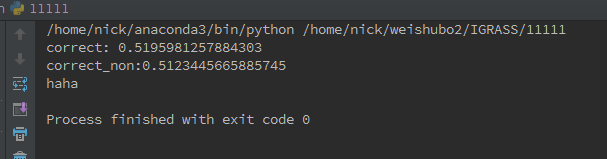
结果表明,稀疏采样后的准确率为51.958%,高于原先的准确率51.234%