#用 pandas 库读取“pollution_us_5city_2006_2010_SO2.csv”文件,查看前五行、后两行。
import pandas as pd
import matplotlib.pyplot as plt
test=pd.read_csv('pollution_us_5city_2006_2010_SO2.csv')
print(test.head(5))
print(test.tail(2))
   ID  State Code  County Code  Site Num                      Address  \
0   1           6           37      1103  1630 N MAIN ST, LOS ANGELES
1   2           6           37      1103  1630 N MAIN ST, LOS ANGELES
2   3           6           37      1103  1630 N MAIN ST, LOS ANGELES
3   4           6           37      1103  1630 N MAIN ST, LOS ANGELES
4   5           6           37      1103  1630 N MAIN ST, LOS ANGELES

        State       County         City Date Local          SO2 Units  \
0  California  Los Angeles  Los Angeles   2006/1/1  Parts per billion
1  California  Los Angeles  Los Angeles   2006/1/1  Parts per billion
2  California  Los Angeles  Los Angeles   2006/1/1  Parts per billion
3  California  Los Angeles  Los Angeles   2006/1/1  Parts per billion
4  California  Los Angeles  Los Angeles   2006/1/2  Parts per billion

   SO2 Mean  SO2 1st Max Value  SO2 1st Max Hour  SO2 AQI
0  2.043478                3.0                 5      4.0
1  2.043478                3.0                 5      4.0
2  2.000000                2.0                 2      NaN
3  2.000000                2.0                 2      NaN
4  2.000000                2.0                 0      3.0
          ID  State Code  County Code  Site Num  \
53218  53219          36           81       124
53219  53220          36           81       124

                                                 Address     State  County  \
53218  Queens College   65-30 Kissena Blvd  Parking L...  New York  Queens
53219  Queens College   65-30 Kissena Blvd  Parking L...  New York  Queens

           City  Date Local          SO2 Units  SO2 Mean  SO2 1st Max Value  \
53218  New York  2010/12/31  Parts per billion   14.8875               16.9
53219  New York  2010/12/31  Parts per billion   14.8875               16.9

       SO2 1st Max Hour  SO2 AQI
53218                 5      NaN
53219                 5      NaN
用 pandas 数据预处理模块将缺失值填充为该列的平均值,删除列 StateCode、County Code、Site Num、Address,并将剩余列导出到 Excel 文件
“pollution_us_5city_2006_2010_SO2.xlsx”。
test.isnull().sum()
mean_cols=test['SO2 AQI'].mean()
test['SO2 AQI'] = test['SO2 AQI'].fillna(mean_cols)
test1=test.drop(['State Code','County Code','Site Num','Address'],axis=1)
test1.to_excel('pollution_us_5city_2006_2010_SO2.xlsx')
读取新的数据集“pollution_us_5city_2006_2010_SO2.xlsx”,并选择字段
City==“New York”的所有数据集,导出为文本文件“pollution_us_NewYork_2006_2010_SO2.txt”,要求数据之间用空格分隔,
每行末尾包含换行符。
test=pd.read_excel('pollution_us_5city_2006_2010_SO2.xlsx')
test2=test.loc[test['City']=="New York"]
test2.to_csv('pollution_us_NewYork_2006_2010_SO2.txt',index=0)
读取文本文件“pollution_us_NewYork_2006_2010_SO2.txt”,并选择字段
Date Local 位于[2007/1/1, 2009/12/31] 区间的所有数据集转存到 CSV 文件
“pollution_us_NewYork_2007_2009_SO2.csv”中。
test=pd.read_csv('pollution_us_NewYork_2006_2010_SO2.txt')
test['Date Local'] = pd.to_datetime(test['Date Local'])
test = test.set_index('Date Local') # 将date设置为index
test=test['2007-01-01':'2009-12-31']
test.to_csv('pollution_us_NewYork_2007_2009_SO2.csv')
读取 CSV 文件“pollution_us_NewYork_2007_2009_SO2.csv”,计算同一个
城市(字段 City)的 SO2 Mean、SO2 1st Max Hour、SO2 AQI 的月均值,
并利用 matplotlib 库可视化显示,要求包括图例、图标题,x 轴刻度以年显
示,y 轴显示刻度值,曲线颜色为红色
test=pd.read_csv('pollution_us_NewYork_2007_2009_SO2.csv')
test.head()
| Date Local | ID | State | County | City | SO2 Units | SO2 Mean | SO2 1st Max Value | SO2 1st Max Hour | SO2 AQI | |
|---|---|---|---|---|---|---|---|---|---|---|
| 0 | 2007-01-01 | 15225 | New York | Bronx | New York | Parts per billion | 6.583333 | 20.0 | 16 | 29.000000 |
| 1 | 2007-01-01 | 15226 | New York | Bronx | New York | Parts per billion | 6.583333 | 20.0 | 16 | 29.000000 |
| 2 | 2007-01-01 | 15227 | New York | Bronx | New York | Parts per billion | 6.562500 | 13.3 | 20 | 10.957132 |
| 3 | 2007-01-01 | 15228 | New York | Bronx | New York | Parts per billion | 6.562500 | 13.3 | 20 | 10.957132 |
| 4 | 2007-01-02 | 15229 | New York | Bronx | New York | Parts per billion | 7.909091 | 19.0 | 20 | 27.000000 |
test['Date Local'] = test['Date Local'].apply(lambda x: pd.Timestamp(x))
# 年份
test['年']=test['Date Local'].apply(lambda x: x.year)
# 月份
test['月']=test['Date Local'].apply(lambda x: x.month)
test=test.drop(['ID','SO2 1st Max Value'],axis=1)
test_num=test.groupby(by=['年','月'],as_index=False).mean()
test_num.info()
<class 'pandas.core.frame.DataFrame'>
Int64Index: 36 entries, 0 to 35
Data columns (total 5 columns):
年                   36 non-null int64
月                   36 non-null int64
SO2 Mean            36 non-null float64
SO2 1st Max Hour    36 non-null float64
SO2 AQI             36 non-null float64
dtypes: float64(3), int64(2)
memory usage: 1.7 KB
test_num['年']=test_num['年'].astype('str')
test_num['月']=test_num['月'].astype('str')
test_num['all']=test_num['年']+'/'+test_num['月']
test_num.columns
Index(['年', '月', 'SO2 Mean', 'SO2 1st Max Hour', 'SO2 AQI', 'all'], dtype='object')
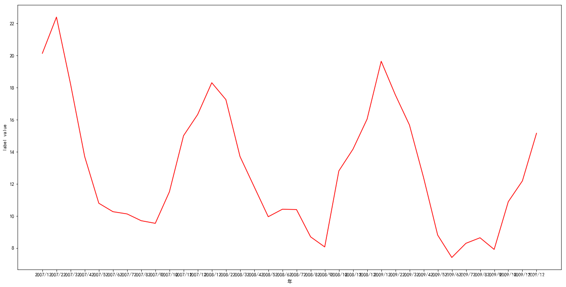
x=test_num['all']
y=test_num['SO2 Mean']
plt.figure(figsize=(20,10))
plt.rcParams['font.sans-serif']=['SimHei'] #用来正常显示中文标签
plt.rcParams['axes.unicode_minus'] = False
plt.plot(x,y, 'r', label='SO2 Mean')
plt.xlabel('年')
plt.ylabel('label value')
Text(0,0.5,'label value')
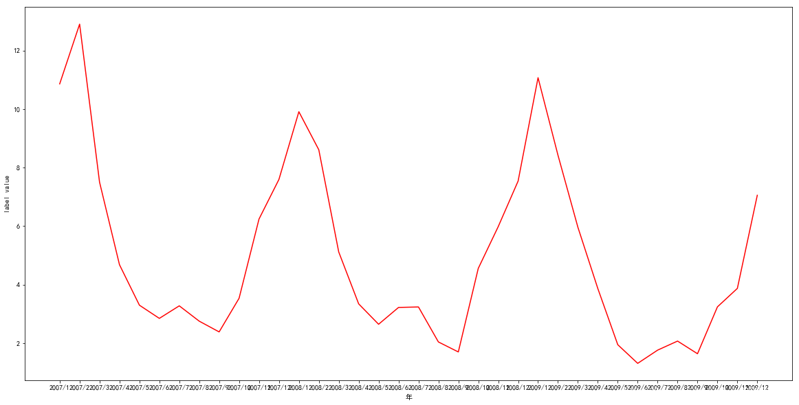
x=test_num['all']
y=test_num['SO2 1st Max Hour']
plt.figure(figsize=(20,10))
plt.rcParams['font.sans-serif']=['SimHei'] #用来正常显示中文标签
plt.rcParams['axes.unicode_minus'] = False
plt.plot(x,y, 'r', label='SO2 Mean')
plt.xlabel('年')
plt.ylabel('label value')
Text(0,0.5,'label value')
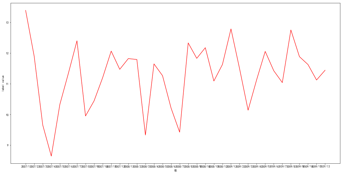
x=test_num['all']
y=test_num['SO2 AQI']
plt.figure(figsize=(20,10))
plt.rcParams['font.sans-serif']=['SimHei'] #用来正常显示中文标签
plt.rcParams['axes.unicode_minus'] = False
plt.plot(x,y, 'r', label='SO2 Mean')
plt.xlabel('年')
plt.ylabel('label value')
Text(0,0.5,'label value')