#3-4-2非矩阵分解
import mglearn
import numpy as np
import matplotlib.pyplot as plt
import pandas as pd
from sklearn.datasets import load_breast_cancer
from sklearn.datasets import make_moons
from sklearn.datasets import make_blobs
from sklearn.datasets import make_circles
from sklearn.datasets import load_iris
from sklearn.datasets import fetch_lfw_people
from sklearn.ensemble import RandomForestClassifier
from sklearn.ensemble import GradientBoostingClassifier
from sklearn.svm import LinearSVC
from sklearn.svm import SVC
from sklearn.neighbors import KNeighborsClassifier
from sklearn.decomposition import NMF
from sklearn.decomposition import PCA
from sklearn.linear_model import LogisticRegression
from sklearn.model_selection import train_test_split
from sklearn.tree import DecisionTreeClassifier
from sklearn.neural_network import MLPClassifier
from sklearn.preprocessing import MinMaxScaler
from sklearn.preprocessing import StandardScaler
from numpy.core.umath_tests import inner1d
from mpl_toolkits.mplot3d import Axes3D,axes3d

mglearn.plots.plot_nmf_illustration()
people = fetch_lfw_people(min_faces_per_person=20,resize=0.7) #灰度图像，按最小比例缩小以加快处理速度
image_shape = people.images[0].shape
mask = np.zeros(people.target.shape,dtype=np.bool)
for target in np.unique(people.target):
    mask[np.where(people.target == target)[0][:50]] = 1  #每个人只取50张照片
x_people = people.data[mask]
y_people = people.target[mask]
x_people = x_people / 255  #将灰度值稳定在0～1之间，而不是0~255之间
x_train,x_test,y_train,y_test = train_test_split(x_people,y_people,stratify=y_people,random_state=0)
mglearn.plots.plot_nmf_faces(x_train,x_test,image_shape)  #使用nmf进行重构

nmf = NMF(n_components=15,random_state=0)
nmf.fit(x_train)
x_train_nmf = nmf.transform(x_train)
x_test_nmf = nmf.transform(x_test)
fix,axes = plt.subplots(3,5,figsize=(15,12),subplot_kw={'xticks':(),'yticks':()})
for i,(component,ax) in enumerate(zip(nmf.components_,axes.ravel())):
    ax.imshow(component.reshape(image_shape))
    ax.set_title("{}.component".format(i))

compn = 3
inds = np.argsort(x_train_nmf[:,compn])[::-1]
fix,axes = plt.subplots(2,5,figsize=(15,8),subplot_kw={'xticks':(),'yticks':()})
for i,(ind,ax) in enumerate(zip(inds,axes.ravel())):
    ax.imshow(x_train[ind].reshape(image_shape))
compn = 7
inds = np.argsort(x_train_nmf[:,compn])[::-1]
fix,axes = plt.subplots(2,5,figsize=(15,8),subplot_kw={'xticks':(),'yticks':()})
for i,(ind,ax) in enumerate(zip(inds,axes.ravel())):
    ax.imshow(x_train[ind].reshape(image_shape))

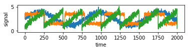
s = mglearn.datasets.make_signals()
plt.figure(figsize=(6,1))
plt.plot(s,'-')
plt.xlabel("time")
plt.ylabel("signal")  #原始信号源

a = np.random.RandomState(0).uniform(size=(100,3))  #随机为100维度
x = np.dot(s,a.T)
print("shape of measurements:{}".format(x.shape))

shape of measurements:(2000, 100)

nmf = NMF(n_components=3,random_state=42)
s_ = nmf.fit_transform(x)
print("recovered signal shape:{}".format(s_.shape))  #还原三维

recovered signal shape:(2000, 3)

pca = PCA(n_components=3)
h = pca.fit_transform(x) 
models = [x,s,s_,h]
names = ['observations(first three measurements)','true sources','nmf recovered signals','pca recovered signals']
fig,axes = plt.subplots(4,figsize=(8,4),gridspec_kw={'hspace':.5},subplot_kw={'xticks':(),'yticks':()})
for model,name,ax in zip(models,names,axes):
    ax.set_title(name)
    ax.plot(model[:,:3],'-')