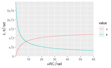
图源于电力电子课本65页——电容滤波的单相不可控整流电路。
f<-function(w,d)
{
  l<-w/sqrt(w^2+1)*exp(-atan(w)/w)*exp(-d/w)
  r<-sin(d)
  return(l-r)
}
w<-seq(0.01,60,0.01)
d<-rep(0,length(w))
s<-rep(0,length(w))
for(i in 1:length(w))
{
  root<-uniroot(f,c(0,pi/2),w=w[i],tol=0.01)
  d[i]<-root$root
  s[i]<-pi-d[i]-atan(w[i])
}

library(ggplot2)
DataSet1<-data.frame(w,value=d,lab=rep("d",length(w)))
DataSet2<-data.frame(w,value=s,lab=rep("s",length(w)))
DataSet <- rbind(DataSet1,DataSet2)

p<-ggplot(data=DataSet,aes(w,value,color=lab))
p+geom_line()+
  scale_colour_hue("value",breaks=c("d","s"),labels=c(expression(delta),expression(theta)))+
  labs(x=(expression(omega*RC/rad)),y=expression(list(delta,theta)/rad))+
  xlim(0,60)+ylim(0,pi)+
  scale_x_continuous(expand = c(0,0))+
  scale_y_continuous(breaks=round(c(0,pi/6,pi/3,pi/2,2*pi/3,5*pi/6,pi),digits=2),
                     labels=expression(0,pi/6,pi/3,pi/2,2*pi/3,5*pi/6,pi),expand = c(0, 0))
练习了:
- 自定义离散色彩标度;
- 修改坐标轴标签;
- 修改坐标范围;
- 修改显示刻度;
- expression数学表达式。