Pytorch|YOWO原理及代码详解(二)

1.正式训练

    if opt.evaluate:
        logging('evaluating ...')
        test(0)
    else:
        for epoch in range(opt.begin_epoch, opt.end_epoch + 1):
            # Train the model for 1 epoch
            train(epoch)

            # Validate the model
            fscore = test(epoch)

            is_best = fscore > best_fscore
            if is_best:
                print("New best fscore is achieved: ", fscore)
                print("Previous fscore was: ", best_fscore)
                best_fscore = fscore

            # Save the model to backup directory
            state = {
                'epoch': epoch,
                'state_dict': model.state_dict(),
                'optimizer': optimizer.state_dict(),
                'fscore': fscore
            }
            save_checkpoint(state, is_best, backupdir, opt.dataset, clip_duration)
            logging('Weights are saved to backup directory: %s' % (backupdir))

为了训练，设置opt.evaluate = False，根据论文(YOWO翻译)(可知ucf24训练5个epoch就可以了。

2. train

查看整个train函数。

    def train(epoch):
        global processed_batches
        t0 = time.time()
        cur_model = model.module
        region_loss.l_x.reset()
        region_loss.l_y.reset()
        region_loss.l_w.reset()
        region_loss.l_h.reset()
        region_loss.l_conf.reset()
        region_loss.l_cls.reset()
        region_loss.l_total.reset()
        train_loader = torch.utils.data.DataLoader(
            dataset.listDataset(basepath, trainlist, dataset_use=dataset_use, shape=(init_width, init_height),
                                shuffle=True,
                                transform=transforms.Compose([
                                    transforms.ToTensor(),
                                ]),
                                train=True,
                                seen=cur_model.seen,
                                batch_size=batch_size,
                                clip_duration=clip_duration,
                                num_workers=num_workers),
            batch_size=batch_size, shuffle=False, **kwargs)

        lr = adjust_learning_rate(optimizer, processed_batches)
        logging('training at epoch %d, lr %f' % (epoch, lr))

        model.train()

        for batch_idx, (data, target) in enumerate(train_loader):
            adjust_learning_rate(optimizer, processed_batches)
            processed_batches = processed_batches + 1

            if use_cuda:
                data = data.cuda()

            optimizer.zero_grad()
            output = model(data)
            region_loss.seen = region_loss.seen + data.data.size(0)
            loss = region_loss(output, target)
            loss.backward()
            optimizer.step()

            # save result every 1000 batches
            if processed_batches % 500 == 0:  # From time to time, reset averagemeters to see improvements
                region_loss.l_x.reset()
                region_loss.l_y.reset()
                region_loss.l_w.reset()
                region_loss.l_h.reset()
                region_loss.l_conf.reset()
                region_loss.l_cls.reset()
                region_loss.l_total.reset()

        t1 = time.time()
        logging('trained with %f samples/s' % (len(train_loader.dataset) / (t1 - t0)))
        print('')

processed_batches是全局变量，存储已经处理的batch数，方便断点继续训练。t0 = time.time()记录当前的时间。region_loss初始化。

2.1 加载训练数据集

训练数据集是放在listDataset类中。listDataset是在dataset.py中，完整代码如下：

class listDataset(Dataset):
    # clip duration = 8, i.e, for each time 8 frames are considered together
    def __init__(self, base, root, dataset_use='ucf101-24', shape=None, shuffle=True,
                 transform=None, target_transform=None, 
                 train=False, seen=0, batch_size=64,
                 clip_duration=16, num_workers=4):
        with open(root, 'r') as file:
            self.lines = file.readlines()
        if shuffle:
            random.shuffle(self.lines)
        self.base_path = base
        self.dataset_use = dataset_use
        self.nSamples  = len(self.lines)
        self.transform = transform
        self.target_transform = target_transform
        self.train = train
        self.shape = shape
        self.seen = seen
        self.batch_size = batch_size
        self.clip_duration = clip_duration
        self.num_workers = num_workers
    def __len__(self):
        return self.nSamples
    def __getitem__(self, index):
        assert index <= len(self), 'index range error'
        imgpath = self.lines[index].rstrip()
        self.shape = (224, 224)
        if self.train: # For Training
            jitter = 0.2
            hue = 0.1
            saturation = 1.5 
            exposure = 1.5
            clip, label = load_data_detection(self.base_path, imgpath,  self.train, self.clip_duration, self.shape, self.dataset_use, jitter, hue, saturation, exposure)
        else: # For Testing
            frame_idx, clip, label = load_data_detection(self.base_path, imgpath, False, self.clip_duration, self.shape, self.dataset_use)
            clip = [img.resize(self.shape) for img in clip]
        if self.transform is not None:
            clip = [self.transform(img) for img in clip]
        # (self.duration, -1) + self.shape = (8, -1, 224, 224)
        clip = torch.cat(clip, 0).view((self.clip_duration, -1) + self.shape).permute(1, 0, 2, 3)
        if self.target_transform is not None:
            label = self.target_transform(label)
        self.seen = self.seen + self.num_workers
        if self.train:
            return (clip, label)
        else:
            return (frame_idx, clip, label)

self.lines存储读去trainlist.txt的文本内容：
在这里插入图片描述
random.shuffle(self.lines)是对其进行打乱。剩下的就是一顿初始化：

2.2 学习率调整

lr = adjust_learning_rate(optimizer, processed_batches)

完整代码：

    def adjust_learning_rate(optimizer, batch):
        lr = learning_rate
        for i in range(len(steps)):
            scale = scales[i] if i < len(scales) else 1
            if batch >= steps[i]:
                lr = lr * scale
                if batch == steps[i]:
                    break
            else:
                break
        for param_group in optimizer.param_groups:
            param_group['lr'] = lr / batch_size
        return lr

学习率是根据steps进行不断调整的，如下：

        ......
        lr = adjust_learning_rate(optimizer, processed_batches)
        logging('training at epoch %d, lr %f' % (epoch, lr))
        model.train()
        for batch_idx, (data, target) in enumerate(train_loader):
            adjust_learning_rate(optimizer, processed_batches)
            processed_batches = processed_batches + 1
        ......

scales和step是ucf24.cfg中进行设置的衰减策略，如下：

在这里插入图片描述

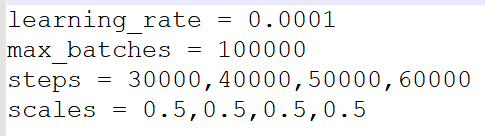
2.3 获取训练数据

这段for batch_idx, (data, target) in enumerate(train_loader):中的data, target是通过listDataset在的def __getitem__(self, index):进行获取的。
在这里插入图片描述
其中：

            jitter = 0.2
            hue = 0.1
            saturation = 1.5 
            exposure = 1.5

是yolov2中用于数据增强的数据，参考YOLOv2 参数详解，其中各项参数意义如下：

jitter：利用数据抖动产生更多数据
hue：色调变化范围
saturation & exposure: 饱和度与曝光变化大小

这部分最关键的是：load_data_detection(self.base_path, imgpath, self.train, self.clip_duration, self.shape, self.dataset_use, jitter, hue, saturation, exposure)
完整代码如下：

def load_data_detection(base_path, imgpath, train, train_dur, shape, dataset_use='ucf101-24', jitter=0.2, hue=0.1, saturation=1.5, exposure=1.5):
    # clip loading and  data augmentation
    # if dataset_use == 'ucf101-24':
    #     base_path = "/usr/home/sut/datasets/ucf24"
    # else:
    #     base_path = "/usr/home/sut/Tim-Documents/jhmdb/data/jhmdb"
    im_split = imgpath.split('/')
    num_parts = len(im_split)
    im_ind = int(im_split[num_parts-1][0:5])
    labpath = os.path.join(base_path, 'labels', im_split[0], im_split[1] ,'{:05d}.txt'.format(im_ind))
    img_folder = os.path.join(base_path, 'rgb-images', im_split[0], im_split[1])
    if dataset_use == 'ucf101-24':
        max_num = len(os.listdir(img_folder))
    else:
        max_num = len(os.listdir(img_folder)) - 1
    clip = []
    ### We change downsampling rate throughout training as a ###
    ### temporal augmentation, which brings around 1-2 frame ###
    ### mAP. During test time it is set to 1.                ###
    d = 1 
    if train:
        d = random.randint(1, 2)
    for i in reversed(range(train_dur)):
        # make it as a loop
        i_temp = im_ind - i * d
        while i_temp < 1:
            i_temp = max_num + i_temp
        while i_temp > max_num:
            i_temp = i_temp - max_num
        if dataset_use == 'ucf101-24':
            path_tmp = os.path.join(base_path, 'rgb-images', im_split[0], im_split[1] ,'{:05d}.jpg'.format(i_temp))
        else:
            path_tmp = os.path.join(base_path, 'rgb-images', im_split[0], im_split[1] ,'{:05d}.png'.format(i_temp))
        clip.append(Image.open(path_tmp).convert('RGB'))
    if train: # Apply augmentation
        clip,flip,dx,dy,sx,sy = data_augmentation(clip, shape, jitter, hue, saturation, exposure)
        label = fill_truth_detection(labpath, clip[0].width, clip[0].height, flip, dx, dy, 1./sx, 1./sy)
        label = torch.from_numpy(label)
    else: # No augmentation
        label = torch.zeros(50*5)
        try:
            tmp = torch.from_numpy(read_truths_args(labpath, 8.0/clip[0].width).astype('float32'))
        except Exception:
            tmp = torch.zeros(1,5)
        tmp = tmp.view(-1)
        tsz = tmp.numel()
        if tsz > 50*5:
            label = tmp[0:50*5]
        elif tsz > 0:
            label[0:tsz] = tmp
    if train:
        return clip, label
    else:
        return im_split[0] + '_' +im_split[1] + '_' + im_split[2], clip, label

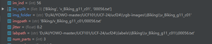
通过把路径进行分割：im_split = imgpath.split('/')，来找到标注labpath和对应的文件夹img_folder。
在这里插入图片描述
“在整个训练过程中，改变下采样率作为一个时间增量，得到1-2帧左右的图像。在测试期间，它被设置为1。”这个下采样率是指帧与帧之间的采样距离，如果d=2，则没隔两帧读取数据，依此类推。

    d = 1 
    if train:
        d = random.randint(1, 2)

这个train_dur对应的参数是self.clip_duration，剪辑持续时间，默认设置的是16。im_ind（在上述图片中可以看到，是56）是标注是整个视频（图像，视频被切割成一张张的图像）序列中的ID。

        i_temp = im_ind - i * d
        while i_temp < 1:
            i_temp = max_num + i_temp
        while i_temp > max_num:
            i_temp = i_temp - max_num

上述代码是为了现在i_temp有效，如果溢出，则使用循环序列。
path_tmp则是获取对应帧的图像，如下：
在这里插入图片描述
clip.append(Image.open(path_tmp).convert('RGB'))将其转换成RGB模式，添加到序列clip中。
在训练的过程中还会使用数据增强来扩充数据集：

    if train: # Apply augmentation
        clip,flip,dx,dy,sx,sy = data_augmentation(clip, shape, jitter, hue, saturation, exposure)
        label = fill_truth_detection(labpath, clip[0].width, clip[0].height, flip, dx, dy, 1./sx, 1./sy)
        label = torch.from_numpy(label)

data_augmentation完整代码如下：

def data_augmentation(clip, shape, jitter, hue, saturation, exposure):
    # Initialize Random Variables
    oh = clip[0].height  
    ow = clip[0].width
    dw =int(ow*jitter)
    dh =int(oh*jitter)
    pleft  = random.randint(-dw, dw)
    pright = random.randint(-dw, dw)
    ptop   = random.randint(-dh, dh)
    pbot   = random.randint(-dh, dh)
    swidth =  ow - pleft - pright
    sheight = oh - ptop - pbot
    sx = float(swidth)  / ow
    sy = float(sheight) / oh 
    dx = (float(pleft)/ow)/sx
    dy = (float(ptop) /oh)/sy
    flip = random.randint(1,10000)%2
    dhue = random.uniform(-hue, hue)
    dsat = rand_scale(saturation)
    dexp = rand_scale(exposure)
    # Augment
    cropped = [img.crop((pleft, ptop, pleft + swidth - 1, ptop + sheight - 1)) for img in clip]
    sized = [img.resize(shape) for img in cropped]
    if flip: 
        sized = [img.transpose(Image.FLIP_LEFT_RIGHT) for img in sized]
    clip = [random_distort_image(img, dhue, dsat, dexp) for img in sized]
    return clip, flip, dx, dy, sx, sy

关于数据增强，这里有几个参数是yolov2中的，上述已经讲过，即是对图像进行抖动，改变色调、饱和度以及曝光度，并进行尺度归一化，缩放为 $224 \times 224$ 。
pleft和ptop是靠左（向右），靠上（向下）的偏移量，swidth和sheight是数据抖动后的宽和高，通过这些参数进行裁剪，cropped = [img.crop((pleft, ptop, pleft + swidth - 1, ptop + sheight - 1)) for img in clip]。
并进一步尺度归一化：sized = [img.resize(shape) for img in cropped]。
如果标志位flip为true，则还会进行水平翻转：sized = [img.transpose(Image.FLIP_LEFT_RIGHT) for img in sized]。
由于图像以及增强了，那么对应的标注label也需要进行对应的改变：label = fill_truth_detection(labpath, clip[0].width, clip[0].height, flip, dx, dy, 1./sx, 1./sy)。由于图像增强，主要是图像的偏移以及方式，所以对应标签的变化需要知道图像是否水平翻转，以及图像的偏移量和放缩量，即flip, dx, dy, 1./sx, 1./sy。查看完整代码：

def fill_truth_detection(labpath, w, h, flip, dx, dy, sx, sy):
    max_boxes = 50
    label = np.zeros((max_boxes,5))
    if os.path.getsize(labpath):
        bs = np.loadtxt(labpath)
        if bs is None:
            return label
        bs = np.reshape(bs, (-1, 5))
        for i in range(bs.shape[0]):
            cx = (bs[i][1] + bs[i][3]) / (2 * 320)
            cy = (bs[i][2] + bs[i][4]) / (2 * 240)
            imgw = (bs[i][3] - bs[i][1]) / 320
            imgh = (bs[i][4] - bs[i][2]) / 240
            bs[i][0] = bs[i][0] - 1
            bs[i][1] = cx
            bs[i][2] = cy
            bs[i][3] = imgw
            bs[i][4] = imgh
        cc = 0
        for i in range(bs.shape[0]):
            x1 = bs[i][1] - bs[i][3]/2
            y1 = bs[i][2] - bs[i][4]/2
            x2 = bs[i][1] + bs[i][3]/2
            y2 = bs[i][2] + bs[i][4]/2            
            x1 = min(0.999, max(0, x1 * sx - dx)) 
            y1 = min(0.999, max(0, y1 * sy - dy)) 
            x2 = min(0.999, max(0, x2 * sx - dx))
            y2 = min(0.999, max(0, y2 * sy - dy))
            bs[i][1] = (x1 + x2)/2
            bs[i][2] = (y1 + y2)/2
            bs[i][3] = (x2 - x1)
            bs[i][4] = (y2 - y1)
            if flip:
                bs[i][1] =  0.999 - bs[i][1] 
            if bs[i][3] < 0.001 or bs[i][4] < 0.001:
                continue
            label[cc] = bs[i]
            cc += 1
            if cc >= 50:
                break
    label = np.reshape(label, (-1))
    return label

根据代码，可以推断label中的标注是 $[num_class, x_{min}, y_{min},x_{max},y_{max}]$ 的格式。

            cx = (bs[i][1] + bs[i][3]) / (2 * 320)
            cy = (bs[i][2] + bs[i][4]) / (2 * 240)
            imgw = (bs[i][3] - bs[i][1]) / 320
            imgh = (bs[i][4] - bs[i][2]) / 240

所以，cx和cy是标注中心在图像中的相对位置（0–1之间），imgw和imgh是标注在图像中的相对宽和高（0–1之间）。 bs[i][0]标识对应的类别， bs[i][0] - 1是因为类别从0开始。因为标注增强，是需要图像的偏移量和放缩量，且都是在0-1之间。
x1，y1，x2和y2则是归一化之后的的 $[x_{min}, y_{min},x_{max},y_{max}]$ 。诸如min(0.999, max(0, x1 * sx - dx))之类的，则是保证坐标是在图像范围内，没有溢出。接下来的bs[i][1]…bs[i][4]则是加上偏移量和放缩量之后的标注信息： $[x_{c}, y_{c},W,H]$ 。如果有水平翻转标志flip，进行翻转。如果宽或者高太小if bs[i][3] < 0.001 or bs[i][4] < 0.001，则跳过。接着，把符合要求的标注放进label 中。在数据增强之后，返回clip和label：

    if train:
        return clip, label

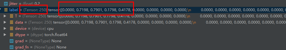
clip是连续帧的图像（224），label是对应的（归一化之后的）目标标签。label的长度为250，是因为默认任务有50个目标（target），每个目标（target）对应五个值， $[class,x_{c}, y_{c},W,H]$ ,如果没有目标，则默认为0。
在这里插入图片描述

在这之后，返回到listDataset类的__getitem__函数中：if self.transform is not None:判断是否需要使用transform进行图像变化，关于transform的使用，可以查看博文：图像预处理——transforms。接下来：clip = torch.cat(clip, 0).view((self.clip_duration, -1) + self.shape).permute(1, 0, 2, 3)则是把连续采样的16帧图像进行拼接，并调整其shape，按照格式： $[Channel,Depth,Height,Weight]$ ，即通道、深度、高和宽，这是为了和torch.nn.Conv3D对应起来，可以看一下clip的shape：
在这里插入图片描述
是满足预期的，通道3，深度16，高224和宽224。接下来通过下述代码，返回数据。

        if self.train:
            return (clip, label)

2.4 loss计算与反向传播

在获取到训练数据和标注之后，则是进行loss计算和反向传播优化：

        for batch_idx, (data, target) in enumerate(train_loader):
            adjust_learning_rate(optimizer, processed_batches)
            processed_batches = processed_batches + 1

            if use_cuda:
                data = data.cuda()

            optimizer.zero_grad()
            output = model(data)
            region_loss.seen = region_loss.seen + data.data.size(0)
            loss = region_loss(output, target)
            loss.backward()
            optimizer.step()

            # save result every 1000 batches
            if processed_batches % 500 == 0:  # From time to time, reset averagemeters to see improvements
                region_loss.l_x.reset()
                region_loss.l_y.reset()
                region_loss.l_w.reset()
                region_loss.l_h.reset()
                region_loss.l_conf.reset()
                region_loss.l_cls.reset()
                region_loss.l_total.reset()

        t1 = time.time()
        logging('trained with %f samples/s' % (len(train_loader.dataset) / (t1 - t0)))
        print('')

每一次迭代，都使用adjust_learning_rate，觉得是否调整学习率。下在看下模型前向传播的tensor的shape变化：output = model(data)。这里data的shape为： $[4,3,16,224,224]$ ,其中的4是batch size，每批有四个数据。现在进入（step into）查看，到了YOWO的forward函数中：

    def forward(self, input):
        x_3d = input # Input clip
        x_2d = input[:, :, -1, :, :] # Last frame of the clip that is read

        x_2d = self.backbone_2d(x_2d)
        x_3d = self.backbone_3d(x_3d)
        x_3d = torch.squeeze(x_3d, dim=2)

        x = torch.cat((x_3d, x_2d), dim=1)
        x = self.cfam(x)

        out = self.conv_final(x)

        return out

x_3d是对应整个视频，而x_2d只是对应视频的最好一帧（上面在生成数据的时候讲到，是根据标注的图片，向前采样，所以x_2d是整个视频序列的最后一帧）。整个流程如下：

x_2d输入到2d网络中：x_2d = self.backbone_2d(x_2d)，输出的shape为 $4 \times 425 \times 7 \times 7$ ,这个是yolov2的预测机制，把图像分成 $7 \times 7$ 大小的grid cell，每个grid cell使用5个anchor预测80个类别的坐标，这就是425的由来，即 $5 \times (5 + 80)$ 。
x_3d输入到3d网络中：x_3d = self.backbone_3d(x_3d)，输出的shape为 $4 \times 2048 \times1\times 7 \times 7$ 。
按照论文的要求是需要把x_3d和x_2d按通道拼接，但是x_3d多了一个维度（depth），所以使用x_3d = torch.squeeze(x_3d, dim=2)压缩维度。
再使用x = torch.cat((x_3d, x_2d), dim=1)进行通道拼接。
接着再输入CFAM模块x = self.cfam(x)，得到输出x，其shape为 $4 \times 1024 \times 7 \times 7$
最后再使用一个卷积层，得到行为理解的时空定位：out = self.conv_final(x)，其中：self.conv_final = nn.Conv2d(1024, 5*(opt.n_classes+4+1), kernel_size=1, bias=False)，其中opt.n_classes = 24，即实现对行为理解的24分类。最后输出的out的shape为： $4 \times 145\times 7 \times 7$ 。

通过上述分析，了解到模型中的output，即上文out，的由来。接下来，便是loss的计算：loss = region_loss(output, target)。进入（step into）其中进行查看，即RegionLoss类的forward函数：

    def forward(self, output, target):
        # output : B*A*(4+1+num_classes)*H*W
        # B: number of batches
        # A: number of anchors
        # 4: 4 parameters for each bounding box
        # 1: confidence score
        # num_classes
        # H: height of the image (in grids)
        # W: width of the image (in grids)
        # for each grid cell, there are A*(4+1+num_classes) parameters
        t0 = time.time()
        nB = output.data.size(0)
        nA = self.num_anchors
        nC = self.num_classes
        nH = output.data.size(2)
        nW = output.data.size(3)

        # resize the output (all parameters for each anchor can be reached)
        output   = output.view(nB, nA, (5+nC), nH, nW)
        # anchor's parameter tx
        x    = torch.sigmoid(output.index_select(2, Variable(torch.cuda.LongTensor([0]))).view(nB, nA, nH, nW))
        # anchor's parameter ty
        y    = torch.sigmoid(output.index_select(2, Variable(torch.cuda.LongTensor([1]))).view(nB, nA, nH, nW))
        # anchor's parameter tw
        w    = output.index_select(2, Variable(torch.cuda.LongTensor([2]))).view(nB, nA, nH, nW)
        # anchor's parameter th
        h    = output.index_select(2, Variable(torch.cuda.LongTensor([3]))).view(nB, nA, nH, nW)
        # confidence score for each anchor
        conf = torch.sigmoid(output.index_select(2, Variable(torch.cuda.LongTensor([4]))).view(nB, nA, nH, nW))
        # anchor's parameter class label
        cls  = output.index_select(2, Variable(torch.linspace(5,5+nC-1,nC).long().cuda()))
        # resize the data structure so that for every anchor there is a class label in the last dimension
        cls  = cls.view(nB*nA, nC, nH*nW).transpose(1,2).contiguous().view(nB*nA*nH*nW, nC)
        t1 = time.time()

        # for the prediction of localization of each bounding box, there exist 4 parameters (tx, ty, tw, th)
        pred_boxes = torch.cuda.FloatTensor(4, nB*nA*nH*nW)
        # tx and ty
        grid_x = torch.linspace(0, nW-1, nW).repeat(nH,1).repeat(nB*nA, 1, 1).view(nB*nA*nH*nW).cuda()
        grid_y = torch.linspace(0, nH-1, nH).repeat(nW,1).t().repeat(nB*nA, 1, 1).view(nB*nA*nH*nW).cuda()
        # for each anchor there are anchor_step variables (with the structure num_anchor*anchor_step)
        # for each row(anchor), the first variable is anchor's width, second is anchor's height
        # pw and ph
        anchor_w = torch.Tensor(self.anchors).view(nA, self.anchor_step).index_select(1, torch.LongTensor([0])).cuda()
        anchor_h = torch.Tensor(self.anchors).view(nA, self.anchor_step).index_select(1, torch.LongTensor([1])).cuda()
        # for each pixel (grid) repeat the above process (obtain width and height of each grid)
        anchor_w = anchor_w.repeat(nB, 1).repeat(1, 1, nH*nW).view(nB*nA*nH*nW)
        anchor_h = anchor_h.repeat(nB, 1).repeat(1, 1, nH*nW).view(nB*nA*nH*nW)
        # prediction of bounding box localization
        # x.data and y.data: top left corner of the anchor
        # grid_x, grid_y: tx and ty predictions made by yowo

        x_data = x.data.view(-1)
        y_data = y.data.view(-1)
        w_data = w.data.view(-1)
        h_data = h.data.view(-1)

        pred_boxes[0] = x_data + grid_x    # bx
        pred_boxes[1] = y_data + grid_y    # by
        pred_boxes[2] = torch.exp(w_data) * anchor_w    # bw
        pred_boxes[3] = torch.exp(h_data) * anchor_h    # bh
        # the size -1 is inferred from other dimensions
        # pred_boxes (nB*nA*nH*nW, 4)
        pred_boxes = convert2cpu(pred_boxes.transpose(0,1).contiguous().view(-1,4))
        t2 = time.time()

        nGT, nCorrect, coord_mask, conf_mask, cls_mask, tx, ty, tw, th, tconf, tcls = build_targets(pred_boxes, target.data, self.anchors, nA, nC, \
                                                               nH, nW, self.noobject_scale, self.object_scale, self.thresh, self.seen)
        cls_mask = (cls_mask == 1)
        #  keep those with high box confidence scores (greater than 0.25) as our final predictions
        nProposals = int((conf > 0.25).sum().data.item())

        tx    = Variable(tx.cuda())
        ty    = Variable(ty.cuda())
        tw    = Variable(tw.cuda())
        th    = Variable(th.cuda())
        tconf = Variable(tconf.cuda())
        tcls = Variable(tcls.view(-1)[cls_mask.view(-1)].long().cuda())

        coord_mask = Variable(coord_mask.cuda())
        conf_mask  = Variable(conf_mask.cuda().sqrt())
        cls_mask   = Variable(cls_mask.view(-1, 1).repeat(1,nC).cuda())
        cls        = cls[cls_mask].view(-1, nC)  

        t3 = time.time()

        # losses between predictions and targets (ground truth)
        # In total 6 aspects are considered as losses: 
        # 4 for bounding box location, 2 for prediction confidence and classification seperately
        loss_x = self.coord_scale * nn.SmoothL1Loss(reduction='sum')(x*coord_mask, tx*coord_mask)/2.0
        loss_y = self.coord_scale * nn.SmoothL1Loss(reduction='sum')(y*coord_mask, ty*coord_mask)/2.0
        loss_w = self.coord_scale * nn.SmoothL1Loss(reduction='sum')(w*coord_mask, tw*coord_mask)/2.0
        loss_h = self.coord_scale * nn.SmoothL1Loss(reduction='sum')(h*coord_mask, th*coord_mask)/2.0
        loss_conf = nn.MSELoss(reduction='sum')(conf*conf_mask, tconf*conf_mask)/2.0

        # try focal loss with gamma = 2
        FL = FocalLoss(class_num=24, gamma=2, size_average=False)
        loss_cls = self.class_scale * FL(cls, tcls)

        # sum of loss
        loss = loss_x + loss_y + loss_w + loss_h + loss_conf + loss_cls
        #print(loss)
        t4 = time.time()

        self.l_x.update(loss_x.data.item(), self.batch)
        self.l_y.update(loss_y.data.item(), self.batch)
        self.l_w.update(loss_w.data.item(), self.batch)
        self.l_h.update(loss_h.data.item(), self.batch)
        self.l_conf.update(loss_conf.data.item(), self.batch)
        self.l_cls.update(loss_cls.data.item(), self.batch)
        self.l_total.update(loss.data.item(), self.batch)


        if False:
            print('-----------------------------------')
            print('        activation : %f' % (t1 - t0))
            print(' create pred_boxes : %f' % (t2 - t1))
            print('     build targets : %f' % (t3 - t2))
            print('       create loss : %f' % (t4 - t3))
            print('             total : %f' % (t4 - t0))
        print('%d: nGT %d, recall %d, proposals %d, loss: x %.2f(%.2f), '
              'y %.2f(%.2f), w %.2f(%.2f), h %.2f(%.2f), conf %.2f(%.2f), '
              'cls %.2f(%.2f), total %.2f(%.2f)'
               % (self.seen, nGT, nCorrect, nProposals, self.l_x.val, self.l_x.avg,
                self.l_y.val, self.l_y.avg, self.l_w.val, self.l_w.avg,
                self.l_h.val, self.l_h.avg, self.l_conf.val, self.l_conf.avg,
                self.l_cls.val, self.l_cls.avg, self.l_total.val, self.l_total.avg))
        return loss

nB是batch size，nA是anchor数，nC是类别数，nH是特征图feature map，即output，的高，同理，nW是宽。output = output.view(nB, nA, (5+nC), nH, nW)讲output的shape进行重塑。
接下来的x = torch.sigmoid(output.index_select(2, Variable(torch.cuda.LongTensor([0]))).view(nB, nA, nH, nW)) 到conf = torch.sigmoid(output.index_select(2, Variable(torch.cuda.LongTensor([4]))).view(nB, nA, nH, nW))，则是分别得到每个anchor的预测的x，y，w，h和confidence(置信度得分)。cls = output.index_select(2, Variable(torch.linspace(5,5+nC-1,nC).long().cuda()))则是得到每个anchor在每一个gird cell上的类别预测结构，其shape为： $4\times 5\times 24\times 7\times 7$ 。接下来调整数据结构的大小，以便在最后一个维度中为每个锚（anchor）都有一个类（class）标签：cls = cls.view(nB*nA, nC, nH*nW).transpose(1,2).contiguous().view(nB*nA*nH*nW, nC)，现在的shape为 $980 \times 24$ ，其中 $980 = 4\times 5 \times 7 \times 7$ ,表示有980个anchor。
对于每个边界框的定位预测，有4个参数（tx，ty，tw，th）。接下来生成grid cell的坐标索引，查看grid_x和grid_y:
在这里插入图片描述
一共980个anchor，grid_x和grid_y分别对应每个anchor的x和y的索引，即【0，0】、【0，1】…【0，6】、【1，0】…
接下来是获取cfg文件中anchor的宽和高，即anchor_w和anchor_h。下面的代码则是把cfg中每个anchor的宽和高分别映射到那980个anchor中：

        anchor_w = anchor_w.repeat(nB, 1).repeat(1, 1, nH*nW).view(nB*nA*nH*nW)
        anchor_h = anchor_h.repeat(nB, 1).repeat(1, 1, nH*nW).view(nB*nA*nH*nW)

查看shape：
在这里插入图片描述

为了和980个anchor对应起来，把x，y，w和h，拉平（flatten），生成对应的x_data,y_data,w_data和h_data。加上偏移量和放缩量，得到预测框的位置：

        pred_boxes[0] = x_data + grid_x    # bx
        pred_boxes[1] = y_data + grid_y    # by
        pred_boxes[2] = torch.exp(w_data) * anchor_w    # bw
        pred_boxes[3] = torch.exp(h_data) * anchor_h    # bh

如果这里看不懂，可以查看一下yolov2的论文，关于边界框预测的机制，即下图：
在这里插入图片描述
接下来把pred_boxes放在cpu上，并重塑其shape为 $(nB*nA*nH*nW, 4)$ 。
然后代码进行计算：nGT, nCorrect, coord_mask, conf_mask, cls_mask, tx, ty, tw, th, tconf, tcls = build_targets(pred_boxes, target.data, self.anchors, nA, nC, nH, nW, self.noobject_scale, self.object_scale, self.thresh, self.seen)，查看函数build_targets，完整代码如下：

def build_targets(pred_boxes, target, anchors, num_anchors, num_classes, nH, nW, noobject_scale, object_scale, sil_thresh, seen):
    # nH, nW here are number of grids in y and x directions (7, 7 here)
    nB = target.size(0) # batch size
    nA = num_anchors    # 5 for our case
    nC = num_classes
    anchor_step = len(anchors)//num_anchors
    conf_mask  = torch.ones(nB, nA, nH, nW) * noobject_scale
    coord_mask = torch.zeros(nB, nA, nH, nW)
    cls_mask   = torch.zeros(nB, nA, nH, nW)
    tx         = torch.zeros(nB, nA, nH, nW) 
    ty         = torch.zeros(nB, nA, nH, nW) 
    tw         = torch.zeros(nB, nA, nH, nW) 
    th         = torch.zeros(nB, nA, nH, nW) 
    tconf      = torch.zeros(nB, nA, nH, nW)
    tcls       = torch.zeros(nB, nA, nH, nW) 

    # for each grid there are nA anchors
    # nAnchors is the number of anchor for one image
    nAnchors = nA*nH*nW
    nPixels  = nH*nW
    # for each image
    for b in xrange(nB):
        # get all anchor boxes in one image
        # (4 * nAnchors)
        cur_pred_boxes = pred_boxes[b*nAnchors:(b+1)*nAnchors].t()
        # initialize iou score for each anchor
        cur_ious = torch.zeros(nAnchors)
        for t in xrange(50):
            # for each anchor 4 coordinate parameters, already in the coordinate system for the whole image
            # this loop is for anchors in each image
            # for each anchor 5 parameters are available (class, x, y, w, h)
            if target[b][t*5+1] == 0:
                break
            gx = target[b][t*5+1]*nW
            gy = target[b][t*5+2]*nH
            gw = target[b][t*5+3]*nW
            gh = target[b][t*5+4]*nH
            # groud truth boxes
            cur_gt_boxes = torch.FloatTensor([gx,gy,gw,gh]).repeat(nAnchors,1).t()
            # bbox_ious is the iou value between orediction and groud truth
            cur_ious = torch.max(cur_ious, bbox_ious(cur_pred_boxes, cur_gt_boxes, x1y1x2y2=False))
        # if iou > a given threshold, it is seen as it includes an object
        # conf_mask[b][cur_ious>sil_thresh] = 0
        conf_mask_t = conf_mask.view(nB, -1)
        conf_mask_t[b][cur_ious>sil_thresh] = 0
        conf_mask_tt = conf_mask_t[b].view(nA, nH, nW)
        conf_mask[b] = conf_mask_tt

    if seen < 12800:
       if anchor_step == 4:
           tx = torch.FloatTensor(anchors).view(nA, anchor_step).index_select(1, torch.LongTensor([2])).view(1,nA,1,1).repeat(nB,1,nH,nW)
           ty = torch.FloatTensor(anchors).view(num_anchors, anchor_step).index_select(1, torch.LongTensor([2])).view(1,nA,1,1).repeat(nB,1,nH,nW)
       else:
           tx.fill_(0.5)
           ty.fill_(0.5)
       tw.zero_()
       th.zero_()
       coord_mask.fill_(1)

    # number of ground truth
    nGT = 0
    nCorrect = 0
    for b in xrange(nB):
        # anchors for one batch (at least batch size, and for some specific classes, there might exist more than one anchor)
        for t in xrange(50):
            if target[b][t*5+1] == 0:
                break
            nGT = nGT + 1
            best_iou = 0.0
            best_n = -1
            min_dist = 10000
            # the values saved in target is ratios
            # times by the width and height of the output feature maps nW and nH
            gx = target[b][t*5+1] * nW
            gy = target[b][t*5+2] * nH
            gi = int(gx)
            gj = int(gy)
            gw = target[b][t*5+3] * nW
            gh = target[b][t*5+4] * nH
            gt_box = [0, 0, gw, gh]
            for n in xrange(nA):
                # get anchor parameters (2 values)
                aw = anchors[anchor_step*n]
                ah = anchors[anchor_step*n+1]
                anchor_box = [0, 0, aw, ah]
                # only consider the size (width and height) of the anchor box
                iou  = bbox_iou(anchor_box, gt_box, x1y1x2y2=False)
                if anchor_step == 4:
                    ax = anchors[anchor_step*n+2]
                    ay = anchors[anchor_step*n+3]
                    dist = pow(((gi+ax) - gx), 2) + pow(((gj+ay) - gy), 2)
                # get the best anchor form with the highest iou
                if iou > best_iou:
                    best_iou = iou
                    best_n = n
                elif anchor_step==4 and iou == best_iou and dist < min_dist:
                    best_iou = iou
                    best_n = n
                    min_dist = dist

            # then we determine the parameters for an anchor (4 values together)
            gt_box = [gx, gy, gw, gh]
            # find corresponding prediction box
            pred_box = pred_boxes[b*nAnchors+best_n*nPixels+gj*nW+gi]

            # only consider the best anchor box, for each image
            coord_mask[b][best_n][gj][gi] = 1
            cls_mask[b][best_n][gj][gi] = 1
            # in this cell of the output feature map, there exists an object
            conf_mask[b][best_n][gj][gi] = object_scale
            tx[b][best_n][gj][gi] = target[b][t*5+1] * nW - gi
            ty[b][best_n][gj][gi] = target[b][t*5+2] * nH - gj
            tw[b][best_n][gj][gi] = math.log(gw/anchors[anchor_step*best_n])
            th[b][best_n][gj][gi] = math.log(gh/anchors[anchor_step*best_n+1])
            iou = bbox_iou(gt_box, pred_box, x1y1x2y2=False) # best_iou
            # confidence equals to iou of the corresponding anchor
            tconf[b][best_n][gj][gi] = iou
            tcls[b][best_n][gj][gi] = target[b][t*5]
            # if ious larger than 0.5, we justify it as a correct prediction
            if iou > 0.5:
                nCorrect = nCorrect + 1

    # true values are returned
    return nGT, nCorrect, coord_mask, conf_mask, cls_mask, tx, ty, tw, th, tconf, tcls

这个函数用于构建groud truth（标注），显示生成shape为 $nB* nA* nH* nW$ 大小的conf_mask，…,tcls。这个build_targets和我在博文Pytorch | yolov3原理及代码详解（二）提到的基本一致。对每个grid都有nA(5)个anchor,nA是一张图片上使用的anchor数量。
接下来来开始遍历：for b in xrange(nB):，获取每张图片的所有anchor。获取当前的所有的预测框：cur_pred_boxes = pred_boxes[b*nAnchors:(b+1)*nAnchors].t()其shape为 $4*245$ 。一张图上有245个anchor，由 $5*7*7$ 计算而来。对于每个anchor4个坐标参数，已在整个图像的坐标系中。此循环用于每个图像中的anchor：for t in xrange(50):，这个50与建立label时默认最多50个target对应。对于每个anchor，有5个参数可用（class，x，y，w，h）。
根据target，乘以特征图feature map的高(nH)和宽(nW)的系数，得到在 $7*7$ 大小的特征图中的绝对坐标：gx，gy，gw，gh。通过这四个值，即可得到ground truth boxes（标注的边界框）cur_gt_boxes。
接下来计算iou值：cur_ious = torch.max(cur_ious, bbox_ious(cur_pred_boxes, cur_gt_boxes, x1y1x2y2=False))，查看完整代码：

def bbox_ious(boxes1, boxes2, x1y1x2y2=True):
    if x1y1x2y2:
        mx = torch.min(boxes1[0], boxes2[0])
        Mx = torch.max(boxes1[2], boxes2[2])
        my = torch.min(boxes1[1], boxes2[1])
        My = torch.max(boxes1[3], boxes2[3])
        w1 = boxes1[2] - boxes1[0]
        h1 = boxes1[3] - boxes1[1]
        w2 = boxes2[2] - boxes2[0]
        h2 = boxes2[3] - boxes2[1]
    else:
        mx = torch.min(boxes1[0]-boxes1[2]/2.0, boxes2[0]-boxes2[2]/2.0)
        Mx = torch.max(boxes1[0]+boxes1[2]/2.0, boxes2[0]+boxes2[2]/2.0)
        my = torch.min(boxes1[1]-boxes1[3]/2.0, boxes2[1]-boxes2[3]/2.0)
        My = torch.max(boxes1[1]+boxes1[3]/2.0, boxes2[1]+boxes2[3]/2.0)
        w1 = boxes1[2]
        h1 = boxes1[3]
        w2 = boxes2[2]
        h2 = boxes2[3]
    uw = Mx - mx
    uh = My - my
    cw = w1 + w2 - uw
    ch = h1 + h2 - uh
    mask = ((cw <= 0) + (ch <= 0) > 0)
    area1 = w1 * h1
    area2 = w2 * h2
    carea = cw * ch
    carea[mask] = 0
    uarea = area1 + area2 - carea
    return carea/uarea

这里的x1y1x2y2设置的是False，计算每个anchor和target的iou值，如果iou>一个给定的阈值，它被视为包含一个对象，则conf_mask置为0（具体见下loss分析），~~下面的一段代码目前没有看懂，可能大概是优化策略~~ ：

    if seen < 12800:
       if anchor_step == 4:
           tx = torch.FloatTensor(anchors).view(nA, anchor_step).index_select(1, torch.LongTensor([2])).view(1,nA,1,1).repeat(nB,1,nH,nW)
           ty = torch.FloatTensor(anchors).view(num_anchors, anchor_step).index_select(1, torch.LongTensor([2])).view(1,nA,1,1).repeat(nB,1,nH,nW)
       else:
           tx.fill_(0.5)
           ty.fill_(0.5)
       tw.zero_()
       th.zero_()
       coord_mask.fill_(1)

接下来分batch，计算ground truth。针对每一批，某些类可能存在多个target。所以会存在循环：for t in xrange(50):。
gx，gy是target 在特征图上的绝对坐标，gi，gj是target在grid cell方格坐标的左上角（这个是yolo的预测机制），gw和gh则是target 在特征图上的绝对宽高。接下来是获取anchor，并计算IOU值，选择具有最高IOU值的anchor，也就是这个iou值计算，是为了选择一个anchor，能和target产生最大的IOU，并选择这个anchor进行预测，即“具体是哪个anchor box预测它，需要在训练中确定，即由那个与ground truth的IOU最大的anchor box预测它”，这个我也在博文在Pytorch | yolov3原理及代码详解（二）中详细分析过，不再赘述。目前anchor_step==4的情况我不能确定是什么模式，大概率是使用4个值来表示一个anchor。
接下来得到targte在特征图上的绝对表示：gt_box = [gx, gy, gw, gh]，选择具有最高IOU值的anchor预测的box：pred_box = pred_boxes[b*nAnchors+best_n*nPixels+gj*nW+gi]。并且，只考虑每个图像的最佳anchor，如果iou值大于阈值，则认为正确预测一个：

            # only consider the best anchor box, for each image
            coord_mask[b][best_n][gj][gi] = 1
            cls_mask[b][best_n][gj][gi] = 1
            # in this cell of the output feature map, there exists an object
            conf_mask[b][best_n][gj][gi] = object_scale
            tx[b][best_n][gj][gi] = target[b][t*5+1] * nW - gi
            ty[b][best_n][gj][gi] = target[b][t*5+2] * nH - gj
            tw[b][best_n][gj][gi] = math.log(gw/anchors[anchor_step*best_n])
            th[b][best_n][gj][gi] = math.log(gh/anchors[anchor_step*best_n+1])
            iou = bbox_iou(gt_box, pred_box, x1y1x2y2=False) # best_iou
            # confidence equals to iou of the corresponding anchor
            tconf[b][best_n][gj][gi] = iou
            tcls[b][best_n][gj][gi] = target[b][t*5]
            # if ious larger than 0.5, we justify it as a correct prediction
            if iou > 0.5:
                nCorrect = nCorrect + 1

计算完毕后，返回到RegionLoss类的forward中，保留那些置信度高（大于0.25）的边界框作为最终预测。接下来把变量放进GPU中。接着便是loss值的计算：

        # losses between predictions and targets (ground truth)
        # In total 6 aspects are considered as losses: 
        # 4 for bounding box location, 2 for prediction confidence and classification seperately
        loss_x = self.coord_scale * nn.SmoothL1Loss(reduction='sum')(x*coord_mask, tx*coord_mask)/2.0
        loss_y = self.coord_scale * nn.SmoothL1Loss(reduction='sum')(y*coord_mask, ty*coord_mask)/2.0
        loss_w = self.coord_scale * nn.SmoothL1Loss(reduction='sum')(w*coord_mask, tw*coord_mask)/2.0
        loss_h = self.coord_scale * nn.SmoothL1Loss(reduction='sum')(h*coord_mask, th*coord_mask)/2.0
        loss_conf = nn.MSELoss(reduction='sum')(conf*conf_mask, tconf*conf_mask)/2.0

        # try focal loss with gamma = 2
        FL = FocalLoss(class_num=24, gamma=2, size_average=False)
        loss_cls = self.class_scale * FL(cls, tcls)

        # sum of loss
        loss = loss_x + loss_y + loss_w + loss_h + loss_conf + loss_cls

这里的损失函数分为3个部分：1.边框损失：（x，y，w，h）。2.置信度损失。3.分类损失。这个损失函数不是原本的yolov2的损失函数。边界框使用的是Smooth L1损失，目标检测中, 如果存在异常点, 如预测4个点, 有一个点偏离很大, L2loss会平方误差, 放大误差, L1对误差的鲁棒性更好。本来coord_mask是为了限制target和best anchor进行loss计算，但是当self.seen < 12800，会被全部置1coord_mask.fill_(1)，我猜测是为了前期训练时，是为了使那些即使不是best iou的anchor也回归到 target上，即有生成Better的anchor，说不定就会有新的best anchor从其中产生，而不是一开始就否定（但是那个tw.zero_()和th.zero_()目前还没有搞懂）。
关于yolov2的loss函数分析具体可见YOLOv2损失函数详解，loss函数的具体形式为：
$\begin{array}{rl}\operatorname{loss}_{t}=\sum_{i=0}^{W} \sum_{j=0}^{H} \sum_{k=0}^{A} & 1_{\text {Max IOU<Thresh} } \lambda_{\text {noobj}} *\left(-b_{i j k}^{o}\right)^{2} \\ & +1_{t<12800} \lambda_{\text {prior}} * \sum_{r \in(x, y, w, h)}\left(\text {prior}_{k}^{r}-b_{i j k}^{r}\right)^{2} \\ + & 1_{k}^{\text {truth}}\left(\lambda_{\text {coord}} * \sum_{r \epsilon(x, y, w, h)}\left(\text {truth}^{r}-b_{i j k}^{r}\right)^{2}\right. \\ & +\lambda_{\text {obj}} *\left(IOU_{\text {truth}}^{k}-b_{i j k}^{o}\right)^{2} \\ & +\lambda_{\text {class}} *\left(\sum_{c=1}^{c}\left(\text {truth}^{c}-b_{i j k}^{c}\right)^{2}\right)\end{array}$
其损失函数可以分为三个部分：

1. $1_{\text {Max lou}<\text {Thresh}} \lambda_{\text {noobj}} *\left(-b_{\text {ijk}}^{o}\right)^{2}$
这个loss是计算background的置信度误差。这里需要计算各个预测框和所有的ground truth之间的IOU值，并且取最大值记作MaxIOU，如果该值小于一定的阈值，YOLOv2论文取了0.6（本代码中的sil_thresh），那么这个预测框就标记为background（可以这么理解：如果所有anchor和target的IOU都太低，说明这些anchor就不适合预测target，那么就应该去预测的是背景background）：conf_mask_t[b][cur_ious>sil_thresh] = 0，同时注意到：conf_mask = torch.ones(nB, nA, nH, nW) * noobject_scale，noobject_scale的取值为1，即 $\lambda_{n o o b j}=1$ 。这句话的含义是指，如果有物体则 $\lambda_{n o o b j}=0$ ，反之，如果没有物体则 $\lambda_{n o o b j}=1$ 。那么第一项就可以写为：
$\lambda_{n o o b j} \sum_{i=0}^{l.h*l.w} \sum_{j=0}^{l \cdot n} 1_{i j}^{n o o b j j}\left(C_{i}-\hat{C}_{i}\right)^{2}+\lambda_{o b j} \sum_{i=0}^{l.h*l.w} \sum_{j=0}^{l.n} 1_{i j}^{o b j}\left(C_{i}-\hat{C}_{i}\right)^{2}$
2. $+1_{t<12800} \lambda_{\text {prior}} * \sum_{r \epsilon(x, y, w, h)}\left(\text {prior}_{k}^{r}-b_{i j k}^{r}\right)^{2}$
这一部分是计算Anchor boxes和预测框的坐标误差，但是只在前12800个iter计算，和我的猜测一样，是为了促进网络学习到Anchor的形状。
3. $\begin{aligned}+1_{k}^{\text {truth}} &\left(\lambda_{\text {coord}} * \sum_{r \epsilon(x, y, w, h)}\left(\text {truth}^{r}-b_{i j k}^{r}\right)^{2}\right.\\ &+\lambda_{o b j} *\left(IOU_{\text {truth}}^{k}-b_{i j k}^{o}\right)^{2} \\ &\left.+\lambda_{\text {class}} *\left(\sum_{c=1}^{c}\left(\text {truth}^{c}-b_{i j k}^{c}\right)^{2}\right)\right) \end{aligned}$
这一部分计算的是和ground truth匹配的预测框各部分的损失总和，包括坐标损失，置信度损失以及分类损失。坐标损失上述已经提过使用了smooth L1 损失。关于置信度损失，增加了一项 $\lambda_{obj}$ 权重系数(代码中的self.object_scale)。对于best anchor进设置conf_mask[b][best_n][gj][gi] = object_scale，本代码其值为5。但是注意到：conf_mask = torch.ones(nB, nA, nH, nW) * noobject_scale，出去被标记为background的anchor被设置为0以外，其余anchor的conf_mask被设置为1。当其为1时，损失是预测框和ground truth的真实IOU值，当其为5时，则应该计算的是best anchor与ground truth，设置为5，应该是增加梯度，倾向于best anchor快速回归到target上面，剩下的则是那些Max_IOU低于阈值的，被设置为0，则进行忽略。最后的类别损失，和上述有点不同，是使用了Focal Loss，来解决类别分类不平衡的问题。

在计算完loss之后，则进行反向传播进行优化，整个训练流程基本分析完毕，剩下的则是test部分。

关于test部分的分析请见：
Pytorch|YOWO原理及代码详解(三)

NotFound1911

发布了82 篇原创文章 · 获赞 62 · 访问量 1万+

私信关注