之前几章所用的MLP、逻辑回归等方法是直接将图像拉成一维向量,这样做有2个很大的问题:
1、相近像素在向量中可能会变得很远,模型很难捕捉到它们之间的空间关系;
2、对于255X255X3的图像,输出层为1000,模型大小可能达到1个多G。
上述的结果显然是我们都不想要的,因此,卷积神经网络(Convolutional Neural Networks, CNN)诞生了。
传统的CNN原理本章不做讨论…
下面使用代码演示一下卷积过程:
1、卷积过程:
# 输入格式为batch*channel*height*width,这里batch和channel都为1
w=nd.arange(4).reshape(1,1,2,2)
b=nd.array([1])
data=nd.arange(9).reshape(1,1,3,3) #相当于图片
out=nd.Convolution(data,w,b,kernel=w.shape[2:],num_filter=w.shape[1])
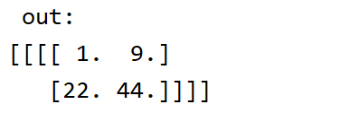
print("input:",data,"\n weight:",w,"\n bias:",b,"\n out:",out)
运行结果:

从上图可以看到,0X0+1X1+2X3+4X3+1=20,正好是out中二维矩阵的第一个结果。
当加上步长、填充方式后:
out=nd.Convolution(data,w,b,kernel=w.shape[2:],num_filter=w.shape[1],stride=(2,2),pad=(1,1))
结果就不一样了…
2、池化
卷积层每次作用在一个窗口上,它对位置信息比较敏感,池化层能很好地缓解这个问题。它跟卷积类似,每次看一个小窗口,然后选出窗口里面最大的元素,或者以平均值的方式输出。
比如一张双通道的图片数据:
data_double=nd.arange(18).reshape(1,2,3,3)  #相当于图片
max_pool=nd.Pooling(data_double,pool_type="max",kernel=(2,2))
avg_pool=nd.Pooling(data_double,pool_type="avg",kernel=(2,2))
print('data:',data_double,'\n max pooling:',max_pool,'\n avg pooling:',avg_pool)
结果:


接下来使用CNN(LeNet)实现图像的分类,下面放上所有代码:
import mxnet.ndarray as nd
import mxnet.autograd as ag
import mxnet.gluon as gn
import mxnet as mx
import matplotlib.pyplot as plt

'''---相关原理代码---'''
'''
# 单通道卷积过程
# 输入格式为batch*channel*height*width,这里batch和channel都为1
w=nd.arange(4).reshape(1,1,2,2)
b=nd.array([1])
data=nd.arange(9).reshape(1,1,3,3)  #相当于图片
# out=nd.Convolution(data,w,b,kernel=w.shape[2:],num_filter=w.shape[1])
# 步长、padding
out=nd.Convolution(data,w,b,kernel=w.shape[2:],num_filter=w.shape[1],stride=(2,2),pad=(1,1))
# print("input:",data,"\n weight:",w,"\n bias:",b,"\n out:",out)
# 池化
data_double=nd.arange(18).reshape(1,2,3,3)  #相当于图片
max_pool=nd.Pooling(data_double,pool_type="max",kernel=(2,2))
avg_pool=nd.Pooling(data_double,pool_type="avg",kernel=(2,2))
print('data:',data_double,'\n max pooling:',max_pool,'\n avg pooling:',avg_pool)
'''

'''---构造卷积神经网络---'''
# 继续使用FashionMNIST
mnist_train = gn.data.vision.FashionMNIST(train=True)
mnist_test = gn.data.vision.FashionMNIST(train=False)


def transform(data, label):
    return data.astype("float32") / 255, label.astype("float32")  # 样本归一化


'''----数据读取----'''
batch_size = 128
transformer = gn.data.vision.transforms.ToTensor()
train_data = gn.data.DataLoader(dataset=mnist_train, batch_size=batch_size, shuffle=True)
test_data = gn.data.DataLoader(dataset=mnist_test, batch_size=batch_size, shuffle=False)

ctx = mx.gpu(0)
# 使用LeNet(不是LeNet-5)(两层卷积+两层全连接)训练mnist数据集
# 1、创建第一个卷积层的w、b ,核大小为5,单通道图片(输入),输出20个特征图
w1 = nd.random_normal(shape=(20, 1, 5, 5), scale=0.01,ctx=ctx)
b1 = nd.random_normal(shape=w1.shape[0], scale=0.01, ctx=ctx)
# 2、创建第二个卷积层的w、b ,核大小为5,输入为20,输出50个特征图
w2 = nd.random_normal(shape=(50, 20, 3, 3), scale=0.01, ctx=ctx)
b2 = nd.random_normal(shape=w2.shape[0], scale=0.01, ctx=ctx)
#  3、全连接层参数------(1250,128)
w3 = nd.random_normal(shape=(1250, 128), scale=0.01, ctx=ctx)
b3 = nd.random_normal(shape=w3.shape[1], scale=0.01, ctx=ctx)
#  4、全连接层参数------(128,10)
w4 = nd.random_normal(shape=(128, 10), scale=0.01, ctx=ctx)
b4 = nd.random_normal(shape=w4.shape[1], scale=0.01, ctx=ctx)

params = [w1, b1, w2, b2, w3, b3, w4, b4]
for param in params:  # 做梯度
    param.attach_grad()


# 定义模型
def cnn_net(X):
    # 第一层卷积+池化
    X = X.as_in_context(w1.context)
    h1_conv = nd.Convolution(data=X.reshape((-1, 1, 28, 28)), weight=w1, bias=b1, kernel=w1.shape[2:],
                             num_filter=w1.shape[0])
    h1_activity = nd.relu(data=h1_conv)  # relu激活
    h1_pool = nd.Pooling(data=h1_activity, kernel=(2, 2), pool_type="max", stride=(2, 2))  # 最大池化
    # 第二层卷积+池化
    h2_conv = nd.Convolution(data=h1_pool, weight=w2, bias=b2, kernel=w2.shape[2:], num_filter=w2.shape[0])
    h2_activity = nd.relu(data=h2_conv)  # relu激活
    h2_pool = nd.Pooling(data=h2_activity, kernel=(2, 2), pool_type="max", stride=(2, 2))  # 最大池化
    # 第一层全连接
    h2 = nd.Flatten(h2_pool)  # 拉成一个batch*一维向量(2D矩阵)
    h3_linear = nd.dot(h2, w3) + b3
    h3 = nd.relu(h3_linear)
    # 第二层全连接
    h4 = nd.dot(h3, w4) + b4
    return h4


# for data,_ in train_data:
#     data=data.reshape(batch_size,1,28,28)
#     break
cross_loss = gn.loss.SoftmaxCrossEntropyLoss()


# 定义准确率
def accuracy(output, label):
    return nd.mean(output.argmax(axis=1) == label).asscalar()


def evaluate_accuracy(data_iter, net):  # 定义测试集准确率
    acc = 0
    for data, label in data_iter:
        data, label = transform(data, label)
        label = label.as_in_context(ctx)
        output = net(data)
        acc += accuracy(output, label)
    return acc / len(data_iter)


# 梯度下降优化器
def SGD(params, lr):
    for pa in params:
        pa[:] = pa - lr * pa.grad  # 参数沿着梯度的反方向走特定距离


# 训练
lr = 0.2
epochs = 10
for epoch in range(epochs):
    train_loss = 0
    train_acc = 0
    for image, y in train_data:
        image, y = transform(image, y)  # 类型转换,数据归一化
        y = y.as_in_context(ctx)
        with ag.record():
            output = cnn_net(image)
            loss = cross_loss(output, y)
        loss.backward()
        # 将梯度做平均,这样学习率不会对batch_size那么敏感
        SGD(params, lr / batch_size)
        train_loss += nd.mean(loss).asscalar()
        train_acc += accuracy(output, y)
        test_acc = evaluate_accuracy(test_data, cnn_net)

    print("Epoch %d, Loss:%f, Train acc:%f, Test acc:%f"
          % (epoch, train_loss / len(train_data), train_acc / len(train_data), test_acc))
训练结果(前几次):

