新闻分类

背景

新闻分类是文本分类中常见的应用场景。传统的分类模式下，往往是通过人工对新闻进行核对，从而将新闻进行分类。但是这种方式效率不高。

• 能够对文本数据进行预处理
• 能够通过Python统计词频，生成词云图
• 能够通过方差分析，进行特征选择。
• 能够根据文本内容，对文本数据进行分类。

1、加载数据集

import numpy as np
import pandas as pd
import matplotlib.pyplot as plt
import matplotlib
import warnings

plt.rcParams["font.family"] = "SimHei"
plt.rcParams["axes.unicode_minus"] = False
plt.rcParams["font.size"] = 15
warnings.filterwarnings("ignore")
%matplotlib inline

news = pd.read_csv("./news.csv", encoding="utf-8")
display(news.head())

2、数据预处理

2.1 缺失值处理

news.info()

##使用新闻标题填充缺失的新闻内容
index = news[news.content.isnull()].index
news["content"][index]=news["headline"][index]  
news.isnull().sum()

2.2 重复值处理

###自定义背景
wc = WordCloud(font_path=r"C:\Windows\Fonts\STFANGSO.ttf", mask=plt.imread("./imgs/map3.jpg"))

plt.figure(figsize=(15,10))
img = wc.generate_from_frequencies(c)
plt.imshow(img)
plt.axis("off")

print(news[news.duplicated()])

news.drop_duplicates(inplace=True)

2.3 文本内容清洗

import re  ####文本的处理 sub调用编译后的正则对象对文本进行处理
re_obj = re.compile(r"['~`!#$%^&*()_+-=|\';:/.,?><~·！@#￥%……&*（）——+-=“：’；、。，？》《{}'：【】《》‘’“”\s]+")

def clear(text):
    return re_obj.sub("", text)
news["content"] = news["content"].apply(clear)

news.sample(10)

2.4 分词

import jieba
def cut_word(text):   ###分词，使用jieba的lcut方法分割词，生成一个列表，
    ####cut()  生成一个生成器， 不占用空间或者说占用很少的空间，使用list()可以转换成列表
    return jieba.lcut(text)

news["content"] = news["content"].apply(cut_word)
news.sample(5)

 2.5 停用词处理

def get_stopword():####删除停用词，就是在文中大量出现，对分类无用的词 降低存储和减少计算时间
    s = set()   ###通过hash处理后的键映射数据    列表则是通过下标的顺序存储映射数据
    with open("./stopword.txt", encoding="utf-8") as f:
        for line in f:
            s.add(line.strip())
    return s         

def remove_stopword(words):
    return [word for word in words if word not in stopword]

stopword = get_stopword()
news["content"] = news["content"].apply(remove_stopword)
news.sample(5)

 3、数据探索

3.1 类别数量分布

###数据探索  描述性分析
###tag统计
t = news["tag"].value_counts()
print(t)
t.plot(kind="bar")

3.2 年份统计

###年份数量分布  指定expand=True生成DataFrame
"""
str.split()有三个参数：第一个参数就是引号里的内容：就是分列的依据，可以是空格，符号，字符串等等。
第二个参数就是前面用到的expand=True，这个参数直接将分列后的结果转换成DataFrame。
第三个参数的n=数字就是限制分列的次数。
如果我想从最右边的开始找分列的依据，可以使用rsplit()，rsplit和split()的用法类似，
一个从右边开始，一个从左边开始。
"""
t = news["date"].str.split("-", expand=True)

t2 = t[0].value_counts()
t2.plot(kind="bar")

3.3 词汇统计

###词汇统计

##词汇频数统计

from itertools import chain
from collections import Counter

li_2d = news["content"].tolist()  ###转二维数组

###二维数组转一维数组
li_1d = list(chain.from_iterable(li_2d))
print(f"词汇总量：{len(li_1d)}")
c = Counter(li_1d)
print(f"不重复词汇数量：{len(c)}")
print(c.most_common(15))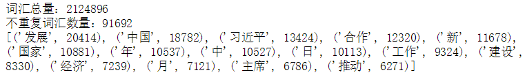

common = c.most_common(15)
d = dict(common)
plt.figure(figsize=(15,5))
plt.bar(d.keys(), d.values())

 3.4 生成词云图

###词云图

from wordcloud import WordCloud

wc = WordCloud(font_path=r"C:\Windows\Fonts\STFANGSO.ttf", width=800, height=600,  background_color='green')
join_word = " ".join(li_1d)   ####词云图需要以空格的格式产生
img = wc.generate(join_word)
plt.figure(figsize=(15,10))
plt.imshow(img)
plt.axis("off")
wc.to_file("wordcloud.png")  

#自定义背景
wc = WordCloud(font_path=r"C:\Windows\Fonts\STFANGSO.ttf", mask=plt.imread("./imgs/map3.jpg"))


plt.figure(figsize=(15,10))
img = wc.generate_from_frequencies(c)
plt.imshow(img)
plt.axis("off")

4、文本向量化

将文本转换为数值特征向量的过程，称为文本向量化。将文本向量化，可以分为如下步骤：

• 对文本分词，拆分成更容易处理的单词
• 将单词转换为数值类型。

4.1 词袋模型

词袋模型是一种能够将文本向量化的方式。在词袋模型中，每一个文档为一个样本，每个不重复的单词为一个特征，单词在文档中出现的次数作为特征值。

4.2 TF-IDF

有些单词，我们不能仅以当前文档中的频数来进行衡量，还要考虑其在语料库中，在其他文档中出现的次数。

TF 词频，指一个单词在文档中出现的次数。

IDF 逆文档频率

计算方式为：

from sklearn.feature_extraction.text import CountVectorizer
count = CountVectorizer()
docs = [
    "Where there is a will, there is a way",
    "There is no royal road to learning."
]
bag = count.fit_transform(docs)
###bag 是一个稀疏的矩阵

print(bag)
###调用toarray()方法，将稀疏矩阵转换成稠密矩阵
print(bag.toarray())

print(count.get_feature_names())###特征
print(count.vocabulary_)  ###单词和编号的映射关系

​
from sklearn.feature_extraction.text import CountVectorizer
count = CountVectorizer()
docs = [
    "Where there is a will, there is a way",
    "There is no royal road to learning."
]
bag = count.fit_transform(docs)
###bag 是一个稀疏的矩阵

print(bag)
###调用toarray()方法，将稀疏矩阵转换成稠密矩阵
print(bag.toarray())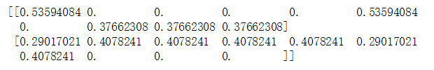

from sklearn.feature_extraction.text import TfidfVectorizer

docs = [
    "Where there is a will, there is a way",
    "There is no royal road to learning."
]
tfidf = TfidfVectorizer()
t = tfidf.fit_transform(docs)
print(t.toarray())

5、建立模型

5.1 构建训练集和测试集

##文本向量化需要传递空格分开的字符串数组类型

def join(text_list):
    return " ".join(text_list)
news["content"] = news["content"].apply(join)

news["tag"] = news["tag"].map({"详细全文": 0, "国内":0, "国际":1})
news["tag"].value_counts()

from sklearn.model_selection import train_test_split

X = news["content"]
y = news["tag"]

X_train, X_test, y_train, y_test = train_test_split(X,y, test_size=0.25)

5.2 特征选择

vec = TfidfVectorizer(ngram_range=(1, 2))####考虑二维的特征 临近的两个特征组合

X_train_vec = vec.fit_transform(X_train)
X_test_vec = vec.transform(X_test)
display(X_train_vec, X_test_vec)

 5.2.1 方差分析

使用词袋模型向量化后，会产生过多的特征，这些特征会对存储与计算造成巨大的压力，同时，并非所有的特征对建模有帮助。

使用方差分析来进行特征选择。

from sklearn.feature_selection import f_classif


#根据y进行分组，计算X中，每个特征的F值与P值
#F值越大，P值越小。
f_classif(X_train_vec, y_train)

from sklearn.feature_selection import SelectKBest

X_train_vec = X_train_vec.astype(np.float32)
X_test_vec = X_test_vec.astype(np.float32)
selector = SelectKBest(f_classif, k=min(20000, X_train_vec.shape[1]))
selector.fit(X_train_vec, y_train)

X_train_vec = selector.transform(X_train_vec)
X_test_vec = selector.transform(X_test_vec)
print(X_train_vec.shape, X_test_vec.shape)

 5.3 逻辑回归

from sklearn.linear_model import LogisticRegression
from sklearn.model_selection import GridSearchCV
from sklearn.metrics import classification_report
param=[{"penalty":["l1","l2"],"C":[0.1,1,10],"solver":["liblinear"]},
      {"penalty":["elasticnet"],"C":[0.1,1,10],"solver":["saga"], "l1_ratio":[0.5]}]

gs = GridSearchCV(estimator=LogisticRegression(), param_grid=param, cv = 5, scoring="f1",n_jobs=-1,verbose=10)

gs.fit(X_train_vec, y_train)

print(gs.best_params_)
y_hat = gs.best_estimator_.predict(X_test_vec)
print(classification_report(y_test,y_hat))

5.4 朴素贝叶斯

from sklearn.naive_bayes import GaussianNB, BernoulliNB, MultinomialNB, ComplementNB

from sklearn.pipeline import Pipeline

from sklearn.preprocessing import FunctionTransformer

###定义函数转换器，将稀疏矩阵转换成稠密矩阵

steps = [("dense",FunctionTransformer(func=lambda X:X.toarray(), accept_sparse=True)),
        ("model", None)]
pipe = Pipeline(steps=steps)
param = {"model":[GaussianNB(), BernoulliNB(), MultinomialNB(), ComplementNB()]}

gs = GridSearchCV(estimator=pipe, param_grid=param, cv=5, scoring="f1", n_jobs=-1,verbose=10)
gs.fit(X_train_vec, y_train)
gs.best_estimator_.predict(X_test_vec)
print(classification_report(y_test, y_hat))