1.世界

1.拓扑图

2. 源码翻译
Hash table based implementation of the <tt>Map</tt> interface.  This
implementation provides all of the optional map operations, and permits
<tt>null</tt> values and the <tt>null</tt> key.  (The <tt>HashMap</tt>
class is roughly equivalent to <tt>Hashtable</tt>, except that it is
unsynchronized and permits nulls.)  This class makes no guarantees as to
the order of the map; in particular, it does not guarantee that the order
will remain constant over time.
基于哈希表实现的映射接口。此实现提供所有可选映射操作,并允许空值和空键。(HashMap类大致相当于Hashtable,只是它是不同步的,并且允许为空。)。该类不保证映射的顺序,特别是,它不能保证订单会随着时间保持不变。
 <p>This implementation provides constant-time performance for the basic
 operations (<tt>get</tt> and <tt>put</tt>), assuming the hash function
 disperses the elements properly among the buckets.  Iteration over
 collection views requires time proportional to the "capacity" of the
 <tt>HashMap</tt> instance (the number of buckets) plus its size (the number
 of key-value mappings).  Thus, it's very important not to set the initial
 capacity too high (or the load factor too low) if iteration performance is
 important.
这个实现为基本操作(get和put)提供了稳定的时间性能,假设hash函数将元素恰当地分散到各个桶中。集合视图的迭代需要与HashMap实例的“容量”(桶的数量)及其大小(键值映射的数量)成比例的时间。因此,如果迭代性能很重要,那么不要将初始容量设置得太高(或负载因子过低)。
<p>An instance of <tt>HashMap</tt> has two parameters that affect its
performance: <i>initial capacity</i> and <i>load factor</i>.  The
<i>capacity</i> is the number of buckets in the hash table, and the initial
capacity is simply the capacity at the time the hash table is created.  The
<i>load factor</i> is a measure of how full the hash table is allowed to
get before its capacity is automatically increased.  When the number of
entries in the hash table exceeds the product of the load factor and the
current capacity, the hash table is <i>rehashed</i> (that is, internal data
structures are rebuilt) so that the hash table has approximately twice the
number of buckets.
HashMap实例有两个影响其性能的参数:初始容量和负载因子。容量是哈希表中的桶数,初始容量就是创建哈希表时的容量。负载因子是衡量在哈希表的容量被自动增加之前,哈希表被允许获得多少满的度量。当哈希表中的条目数超过负载因子和当前容量的乘积时,哈希表将被重新哈希(即重新构建内部数据结构),这样哈希表的桶数大约是桶数的两倍。
<p>As a general rule, the default load factor (.75) offers a good
tradeoff between time and space costs.  Higher values decrease the
space overhead but increase the lookup cost (reflected in most of
the operations of the <tt>HashMap</tt> class, including
<tt>get</tt> and <tt>put</tt>).  The expected number of entries in
the map and its load factor should be taken into account when
setting its initial capacity, so as to minimize the number of
rehash operations.  If the initial capacity is greater than the
maximum number of entries divided by the load factor, no rehash
operations will ever occur.
一般来说,默认的负载因子(0.75)在时间和空间成本之间提供了很好的权衡。较高的值减少了空间开销,但增加了查找成本(反映在HashMap类的大多数操作中,包括get和put)。在设置map的初始容量时,应该考虑map中预期条目的数量及其负载因子,从而最小化rehash操作的数量。如果初始容量大于最大条目数除以负载因子,则不会发生任何重哈希操作。
<p>If many mappings are to be stored in a <tt>HashMap</tt>
instance, creating it with a sufficiently large capacity will allow
the mappings to be stored more efficiently than letting it perform
automatic rehashing as needed to grow the table.  Note that using
many keys with the same {@code hashCode()} is a sure way to slow
down performance of any hash table. To ameliorate impact, when keys
are {@link Comparable}, this class may use comparison order among
keys to help break ties.
如果要将许多映射存储在HashMap实例中,那么使用足够大的容量创建映射将比让映射根据需要执行自动哈希来增长表更有效地存储映射。注意,使用多个具有相同{@code hashCode()}的键肯定会降低任何散列表的性能。为了改善影响,当键是{@link Comparable}时,该类可以使用键之间的比较顺序来帮助断开连接。
 <p><strong>Note that this implementation is not synchronized.</strong>
 If multiple threads access a hash map concurrently, and at least one of
 the threads modifies the map structurally, it <i>must</i> be
 synchronized externally.  (A structural modification is any operation
 that adds or deletes one or more mappings; merely changing the value
 associated with a key that an instance already contains is not a
 structural modification.)  This is typically accomplished by
 synchronizing on some object that naturally encapsulates the map.
注意,这个实现不是同步的。如果多个线程同时访问一个散列映射,并且其中至少有一个线程从结构上修改了映射,那么它必须在外部同步。(结构修改是添加或删除一个或多个映射的任何操作;仅更改与实例已经包含的键关联的值不是结构修改。)这通常是通过在一些自然封装映射的对象上进行同步来实现的。
If no such object exists, the map should be "wrapped" using the
{@link Collections#synchronizedMap Collections.synchronizedMap}
method.  This is best done at creation time, to prevent accidental
unsynchronized access to the map:<pre>
  Map m = Collections.synchronizedMap(new HashMap(...));</pre>
如果不存在这样的对象,则应该使用{@link Collections#synchronizedMap集合’包装’映射。synchronizedMap}方法。这最好在创建时完成,以防止意外的不同步访问地图:
Map m = Collections.synchronizedMap(new HashMap(…));
<p>The iterators returned by all of this class's "collection view methods"
are <i>fail-fast</i>: if the map is structurally modified at any time after
the iterator is created, in any way except through the iterator's own
<tt>remove</tt> method, the iterator will throw a
{@link ConcurrentModificationException}.  Thus, in the face of concurrent
modification, the iterator fails quickly and cleanly, rather than risking
arbitrary, non-deterministic behavior at an undetermined time in the
future.
这个类的所有“collection view methods”返回的迭代器都是快速失败的:如果在创建迭代器之后,以任何方式(除了通过迭代器自己的remove方法)对映射进行结构修改,迭代器将抛出{@link ConcurrentModificationException}。因此,在面对并发修改时,迭代器会快速而干净地失败,而不是在将来某个不确定的时间冒着任意的、不确定的行为的风险。
<p>Note that the fail-fast behavior of an iterator cannot be guaranteed
as it is, generally speaking, impossible to make any hard guarantees in the
presence of unsynchronized concurrent modification.  Fail-fast iterators
throw <tt>ConcurrentModificationException</tt> on a best-effort basis.
Therefore, it would be wrong to write a program that depended on this
exception for its correctness: <i>the fail-fast behavior of iterators
should be used only to detect bugs.</i>
注意,不能保证迭代器的快速故障行为,因为通常来说,在存在非同步并发修改的情况下,不可能做出任何严格的保证。故障快速迭代器以最大的努力抛出ConcurrentModificationException。因此,编写一个依赖于此异常来判断其正确性的程序是错误的:迭代器的快速故障行为应该只用于检测bug。
3.概述
HashMap 最早出现在 JDK 1.2中,底层基于散列算法实现。HashMap 允许 null 键和 null 值,在计算哈键的哈希值时,null 键哈希值为 0。HashMap 并不保证键值对的顺序,这意味着在进行某些操作后,键值对的顺序可能会发生变化。另外,需要注意的是,HashMap 是非线程安全类,在多线程环境下可能会存在问题。
4.原理
HashMap 底层是基于散列算法实现,散列算法分为散列再探测和拉链式。HashMap 则使用了拉链式的散列算法,并在 JDK 1.8 中引入了红黑树优化过长的链表。数据结构示意图如下:

对于拉链式的散列算法,其数据结构是由数组和链表(或树形结构)组成。在进行增删查等操作时,首先要定位到元素的所在桶的位置,之后再从链表中定位该元素。比如我们要查询上图结构中是否包含元素35,步骤如下:
- 定位元素
35所处桶的位置,index = 35 % 16 = 3 - 在
3号桶所指向的链表中继续查找,发现35在链表中。
上面就是 HashMap 底层数据结构的原理,HashMap 基本操作就是对拉链式散列算法基本操作的一层包装。不同的地方在于 JDK 1.8 中引入了红黑树,底层数据结构由数组+链表变为了数组+链表+红黑树,不过本质并未变。好了,原理部分先讲到这,接下来说说源码实现。
5.源码分析
本篇文章所分析的源码版本为 JDK 1.8。与 JDK 1.7 相比,JDK 1.8 对 HashMap 进行了一些优化。比如引入红黑树解决过长链表效率低的问题。重写 resize 方法,移除了 alternative hashing 相关方法,避免重新计算键的 hash 等。不过本篇文章并不打算对这些优化进行分析,本文仅会分析 HashMap 常用的方法及一些重要属性和相关方法。
6.私有变量
6.1 灰色说明
私有变量前面有一些灰色的说明,我们看看是说的什么?
Implementation notes.
This map usually acts as a binned (bucketed) hash table, but
when bins get too large, they are transformed into bins of
TreeNodes, each structured similarly to those in
java.util.TreeMap. Most methods try to use normal bins, but
relay to TreeNode methods when applicable (simply by checking
instanceof a node).  Bins of TreeNodes may be traversed and
used like any others, but additionally support faster lookup
when overpopulated. However, since the vast majority of bins in
normal use are not overpopulated, checking for existence of
tree bins may be delayed in the course of table methods.
实现说明:
这个映射通常充当一个binned (bucketed)哈希表,但是当bins变得太大时,它们会被转换成树节点的bins,每个bins的结构都类似于java.util.TreeMap中的bins。大多数方法都尝试使用普通的bins,但在适用时中继到TreeNode方法(只需检查节点的instanceof)。树节点的存储箱可以像其他存储箱一样被遍历和使用,但是在过度填充时支持更快的查找。但是,由于正常使用的大多数箱子并没有过度填充,所以在表方法的过程中可能会延迟检查树箱子是否存在。
Tree bins (i.e., bins whose elements are all TreeNodes) are
ordered primarily by hashCode, but in the case of ties, if two
elements are of the same "class C implements Comparable<C>",
type then their compareTo method is used for ordering. (We
conservatively check generic types via reflection to validate
this -- see method comparableClassFor).  The added complexity
of tree bins is worthwhile in providing worst-case O(log n)
operations when keys either have distinct hashes or are
orderable, Thus, performance degrades gracefully under
accidental or malicious usages in which hashCode() methods
return values that are poorly distributed, as well as those in
which many keys share a hashCode, so long as they are also
Comparable. (If neither of these apply, we may waste about a
factor of two in time and space compared to taking no
precautions. But the only known cases stem from poor user
programming practices that are already so slow that this makes
little difference.)
树垃圾箱(即。,其元素都是treenode的bin)主要由hashCode排序,但在tie的情况下,如果两个元素具有相同的“class C implementation Comparable”,则键入它们的compareTo方法来排序。(我们通过反射保守地检查泛型类型来验证这一点——请参见comparableClassFor方法)。树的额外复杂性垃圾箱是值得的在提供坏的O (log n)操作键有不同的散列或公开,定货时因此,性能降低优雅地在意外或恶意使用hashCode()方法返回值的差分布,以及许多密钥共享一个hashCode,只要他们也类似。(如果这两种方法都不适用,与不采取预防措施相比,我们可能会浪费大约两倍的时间和空间。但目前所知的唯一案例来自于糟糕的用户编程实践,这些实践已经非常缓慢,以至于没有什么区别。)
Because TreeNodes are about twice the size of regular nodes, we
use them only when bins contain enough nodes to warrant use
(see TREEIFY_THRESHOLD). And when they become too small (due to
removal or resizing) they are converted back to plain bins.  In
usages with well-distributed user hashCodes, tree bins are
rarely used.  Ideally, under random hashCodes, the frequency of
nodes in bins follows a Poisson distribution
(http://en.wikipedia.org/wiki/Poisson_distribution) with a
parameter of about 0.5 on average for the default resizing
threshold of 0.75, although with a large variance because of
resizing granularity. Ignoring variance, the expected
occurrences of list size k are (exp(-0.5) * pow(0.5, k) /
factorial(k)). The first values are:
0:    0.60653066
1:    0.30326533
2:    0.07581633
3:    0.01263606
4:    0.00157952
5:    0.00015795
6:    0.00001316
7:    0.00000094
8:    0.00000006
more: less than 1 in ten million
The root of a tree bin is normally its first node.  However,
sometimes (currently only upon Iterator.remove), the root might
be elsewhere, but can be recovered following parent links
(method TreeNode.root()).
All applicable internal methods accept a hash code as an
argument (as normally supplied from a public method), allowing
them to call each other without recomputing user hashCodes.
Most internal methods also accept a "tab" argument, that is
normally the current table, but may be a new or old one when
resizing or converting.
When bin lists are treeified, split, or untreeified, we keep
them in the same relative access/traversal order (i.e., field
Node.next) to better preserve locality, and to slightly
simplify handling of splits and traversals that invoke
iterator.remove. When using comparators on insertion, to keep a
total ordering (or as close as is required here) across
rebalancings, we compare classes and identityHashCodes as
tie-breakers.
The use and transitions among plain vs tree modes is
complicated by the existence of subclass LinkedHashMap. See
below for hook methods defined to be invoked upon insertion,
removal and access that allow LinkedHashMap internals to
otherwise remain independent of these mechanics. (This also
requires that a map instance be passed to some utility methods
that may create new nodes.)
The concurrent-programming-like SSA-based coding style helps
avoid aliasing errors amid all of the twisty pointer operations.
6.2 构造方法
/**
* The default initial capacity - MUST be a power of two.
* 默认初始容量—必须是2的幂。
*/
static final int DEFAULT_INITIAL_CAPACITY = 1 << 4; // aka 16

/**
* The maximum capacity, used if a higher value is implicitly specified
* by either of the constructors with arguments.
* MUST be a power of two <= 1<<30.
*
* 最大容量,如果较高的值由带参数的任何构造函数隐式指定,则使用该值。必须是2的幂<= 1<<30。
*/
static final int MAXIMUM_CAPACITY = 1 << 30;
/**
* The load factor used when none specified in constructor.
* 构造函数中没有指定时使用的负载因子。
*/
static final float DEFAULT_LOAD_FACTOR = 0.75f;

/**
* The bin count threshold for using a tree rather than list for a
* bin.  Bins are converted to trees when adding an element to a
* bin with at least this many nodes. The value must be greater
* than 2 and should be at least 8 to mesh with assumptions in
* tree removal about conversion back to plain bins upon
* shrinkage.
*
* 使用树(而不是列表)来设置bin计数阈值。当向至少具有这么多节点的bin添加元素时,bin将转换为树。
* 该值必须大于2,并且应该至少为8,以便与树木移除中关于收缩后转换回普通垃圾箱的假设相吻合。
*/
static final int TREEIFY_THRESHOLD = 8;

/**
* The bin count threshold for untreeifying a (split) bin during a
* resize operation. Should be less than TREEIFY_THRESHOLD, and at
* most 6 to mesh with shrinkage detection under removal.
*
* 用于在调整大小操作期间反树化(拆分)bin的bin计数阈值。应小于TREEIFY_THRESHOLD,且最多6个孔配合
* 下进行缩孔检测。
*/
static final int UNTREEIFY_THRESHOLD = 6;

/**
* The smallest table capacity for which bins may be treeified.
* (Otherwise the table is resized if too many nodes in a bin.)
* Should be at least 4 * TREEIFY_THRESHOLD to avoid conflicts
* between resizing and treeification thresholds.
*
* 最小的表容量,其中的箱子可以treeified。(否则,如果一个bin中有太多节点,则会调整表的大小。)应至少为
* 4 * TREEIFY_THRESHOLD,以避免调整大小和treeification阈值之间的冲突。
*/
static final int MIN_TREEIFY_CAPACITY = 64;
7.构造方法
HashMap 的构造方法不多,只有四个。HashMap 构造方法做的事情比较简单,一般都是初始化一些重要变量,比如 loadFactor 和 threshold。而底层的数据结构则是延迟到插入键值对时再进行初始化。HashMap 相关构造方法如下:
 	 /**
     * Constructs an empty <tt>HashMap</tt> with the default initial capacity
     * (16) and the default load factor (0.75).
     * 构造方法 1
     */
    public HashMap() {
        this.loadFactor = DEFAULT_LOAD_FACTOR; // all other fields defaulted
    }

	/**
     * Constructs an empty <tt>HashMap</tt> with the specified initial
     * capacity and the default load factor (0.75).
     *
     * @param  initialCapacity the initial capacity.
     * @throws IllegalArgumentException if the initial capacity is negative.
     * 构造方法 2
     */
    public HashMap(int initialCapacity) {
        this(initialCapacity, DEFAULT_LOAD_FACTOR);
    }


	/**
     * Constructs an empty <tt>HashMap</tt> with the specified initial
     * capacity and load factor.
     *
     * @param  initialCapacity the initial capacity
     * @param  loadFactor      the load factor
     * @throws IllegalArgumentException if the initial capacity is negative
     *         or the load factor is nonpositive
     * 构造方法 3
     */
    public HashMap(int initialCapacity, float loadFactor) {
        if (initialCapacity < 0)
            throw new IllegalArgumentException("Illegal initial capacity: " +
                                               initialCapacity);
        if (initialCapacity > MAXIMUM_CAPACITY)
            initialCapacity = MAXIMUM_CAPACITY;
        if (loadFactor <= 0 || Float.isNaN(loadFactor))
            throw new IllegalArgumentException("Illegal load factor: " +
                                               loadFactor);
        this.loadFactor = loadFactor;
        this.threshold = tableSizeFor(initialCapacity);
    }


    /**
     * Constructs a new <tt>HashMap</tt> with the same mappings as the
     * specified <tt>Map</tt>.  The <tt>HashMap</tt> is created with
     * default load factor (0.75) and an initial capacity sufficient to
     * hold the mappings in the specified <tt>Map</tt>.
     *
     * @param   m the map whose mappings are to be placed in this map
     * @throws  NullPointerException if the specified map is null
     *
     * 构造方法 4
     */
    public HashMap(Map<? extends K, ? extends V> m) {
        this.loadFactor = DEFAULT_LOAD_FACTOR;
        putMapEntries(m, false);
    }
上面4个构造方法中,大家平时用的最多的应该是第一个了。
- 第一个构造方法很简单,仅将 loadFactor 变量设为默认值。
- 构造方法2调用了构造方法3
- 而构造方法3仍然只是设置了一些变量。
- 构造方法4则是将另一个 Map 中的映射拷贝一份到自己的存储结构中来,这个方法不是很常用。
8.初始容量、负载因子、阈值
上面就是对构造方法简单的介绍,构造方法本身并没什么太多东西,所以就不说了。接下来说说构造方法所初始化的几个的变量。
我们在一般情况下,都会使用无参构造方法创建 HashMap。但当我们对时间和空间复杂度有要求的时候,使用默认值有时可能达不到我们的要求,这个时候我们就需要手动调参。在 HashMap 构造方法中,可供我们调整的参数有两个,一个是初始容量 initialCapacity,另一个负载因子 loadFactor。通过这两个设定这两个参数,可以进一步影响阈值大小。但初始阈值 threshold 仅由 initialCapacity 经过移位操作计算得出。他们的作用分别如下:
| 名称 | 用途 |
|---|---|
| initialCapacity | HashMap 初始容量 |
| loadFactor | 负载因子 |
| threshold | 当前 HashMap 所能容纳键值对数量的最大值,超过这个值,则需扩容 |
相关代码如下:
/** The default initial capacity - MUST be a power of two. */
static final int DEFAULT_INITIAL_CAPACITY = 1 << 4;

/** The load factor used when none specified in constructor. */
static final float DEFAULT_LOAD_FACTOR = 0.75f;

final float loadFactor;

/** The next size value at which to resize (capacity * load factor). */
int threshold;
如果大家去看源码,会发现 HashMap 中没有定义 initialCapacity 这个变量。这个也并不难理解,从参数名上可看出,这个变量表示一个初始容量,只是构造方法中用一次,没必要定义一个变量保存。但如果大家仔细看上面 HashMap 的构造方法,会发现存储键值对的数据结构并不是在构造方法里初始化的。这就有个疑问了,既然叫初始容量,但最终并没有用与初始化数据结构,那传这个参数还有什么用呢?这个问题我先不解释,给大家留个悬念,后面会说明。
默认情况下,HashMap初始容量是16,负载因子为 0.75。这里并没有默认阈值,原因是阈值可由容量乘上负载因子计算而来(注释中有说明),即threshold = capacity * loadFactor。但当你仔细看构造方法3时,会发现阈值并不是由上面公式计算而来,而是通过一个方法算出来的。这是不是可以说明 threshold 变量的注释有误呢?还是仅这里进行了特殊处理,其他地方遵循计算公式呢?关于这个疑问,这里也先不说明,后面在分析扩容方法时,再来解释这个问题。接下来,我们来看看初始化 threshold 的方法长什么样的的,源码如下:
   /**
     * Returns a power of two size for the given target capacity.
     */
    static final int tableSizeFor(int cap) {
        int n = cap - 1;
        n |= n >>> 1;
        n |= n >>> 2;
        n |= n >>> 4;
        n |= n >>> 8;
        n |= n >>> 16;
        return (n < 0) ? 1 : (n >= MAXIMUM_CAPACITY) ? MAXIMUM_CAPACITY : n + 1;
    }
上面的代码长的有点不太好看,反正我第一次看的时候不明白它想干啥。不过后来在纸上画画,知道了它的用途。总结起来就一句话:找到大于或等于 cap 的最小2的幂。至于为啥要这样,后面再解释。我们先来看看 tableSizeFor 方法的图解:

上面是 tableSizeFor 方法的计算过程图,这里cap = 536,870,913 = 2<sup>29</sup> + 1,多次计算后,算出n + 1 = 1,073,741,824 = 2<sup>30</sup>。通过图解应该可以比较容易理解这个方法的用途,这里就不多说了。
说完了初始阈值的计算过程,再来说说负载因子(loadFactor)。对于 HashMap 来说,负载因子是一个很重要的参数,该参数反应了 HashMap 桶数组的使用情况(假设键值对节点均匀分布在桶数组中)。通过调节负载因子,可使 HashMap 时间和空间复杂度上有不同的表现。当我们调低负载因子时,HashMap 所能容纳的键值对数量变少。扩容时,重新将键值对存储新的桶数组里,键的键之间产生的碰撞会下降,链表长度变短。此时,HashMap 的增删改查等操作的效率将会变高,这里是典型的拿空间换时间。相反,如果增加负载因子(负载因子可以大于1),HashMap 所能容纳的键值对数量变多,空间利用率高,但碰撞率也高。这意味着链表长度变长,效率也随之降低,这种情况是拿时间换空间。至于负载因子怎么调节,这个看使用场景了。一般情况下,我们用默认值就可以了。
9.查找
HashMap 的查找操作比较简单,查找步骤与原理篇介绍一致,即先定位键值对所在的桶的位置,然后再对链表或红黑树进行查找。通过这两步即可完成查找,该操作相关代码如下:
 /**
     * Implements Map.get and related methods.
     *
     * @param hash hash for key
     * @param key the key
     * @return the node, or null if none
     */
    final Node<K,V> getNode(int hash, Object key) {
        Node<K,V>[] tab; Node<K,V> first, e; int n; K k;
        // 1. 定位键值对所在桶的位置
        if ((tab = table) != null && (n = tab.length) > 0 &&
            (first = tab[(n - 1) & hash]) != null) {
            if (first.hash == hash && // always check first node
                ((k = first.key) == key || (key != null && key.equals(k))))
                return first;
            if ((e = first.next) != null) {
                // 2. 如果 first 是 TreeNode 类型,则调用黑红树查找方法
                if (first instanceof TreeNode)
                    return ((TreeNode<K,V>)first).getTreeNode(hash, key);
                do {
                    // 2. 对链表进行查找
                    if (e.hash == hash &&
                        ((k = e.key) == key || (key != null && key.equals(k))))
                        return e;
                } while ((e = e.next) != null);
            }
        }
        return null;
    }
查找的核心逻辑是封装在 getNode 方法中的,getNode 方法源码我已经写了一些注释,应该不难看懂。我们先来看看查找过程的第一步 - 确定桶位置,其实现代码如下:
// index = (n - 1) & hash
first = tab[(n - 1) & hash]
这里通过(n - 1)& hash即可算出桶的在桶数组中的位置,可能有的朋友不太明白这里为什么这么做,这里简单解释一下。HashMap 中桶数组的大小 length 总是2的幂,此时,(n - 1) & hash 等价于对 length 取余。但取余的计算效率没有位运算高,所以(n - 1) & hash也是一个小的优化。举个例子说明一下吧,假设 hash = 185,n = 16。计算过程示意图如下:

上面的计算并不复杂,这里就不多说了。
在上面源码中,除了查找相关逻辑,还有一个计算 hash 的方法。这个方法源码如下:
 /**
     * Computes key.hashCode() and spreads (XORs) higher bits of hash
     * to lower.  Because the table uses power-of-two masking, sets of
     * hashes that vary only in bits above the current mask will
     * always collide. (Among known examples are sets of Float keys
     * holding consecutive whole numbers in small tables.)  So we
     * apply a transform that spreads the impact of higher bits
     * downward. There is a tradeoff between speed, utility, and
     * quality of bit-spreading. Because many common sets of hashes
     * are already reasonably distributed (so don't benefit from
     * spreading), and because we use trees to handle large sets of
     * collisions in bins, we just XOR some shifted bits in the
     * cheapest possible way to reduce systematic lossage, as well as
     * to incorporate impact of the highest bits that would otherwise
     * never be used in index calculations because of table bounds.
     */
    static final int hash(Object key) {
        int h;
        return (key == null) ? 0 : (h = key.hashCode()) ^ (h >>> 16);
    }
翻译:计算key.hashCode(),并将(XORs)的散列值由高向低扩展。由于该表使用了2的幂掩码,因此仅在当前掩码之上以位为单位变化的散列集总是会发生冲突。(已知的例子包括在小表中保存连续整数的浮点键集。)因此,我们应用一个转换,将更高位的影响向下传播。位扩展的速度、实用性和质量之间存在权衡。因为许多常见的散列集已经合理分布(所以不要受益于传播),因为我们用树来处理大型的碰撞在垃圾箱,我们只是XOR一些改变以最便宜的方式来减少系统lossage,以及将最高位的影响,否则永远不会因为指数计算中使用的表。
测试:
1637079510
看这个方法的逻辑好像是通过位运算重新计算 hash,那么这里为什么要这样做呢?为什么不直接用键的 hashCode 方法产生的 hash 呢?大家先可以思考一下,我把答案写在下面。
这样做有两个好处,我来简单解释一下。我们再看一下上面求余的计算图,图中的 hash 是由键的 hashCode 产生。计算余数时,由于 n 比较小,hash 只有低4位参与了计算,高位的计算可以认为是无效的。这样导致了计算结果只与低位信息有关,高位数据没发挥作用。为了处理这个缺陷,我们可以上图中的 hash 高4位数据与低4位数据进行异或运算,即 hash ^ (hash >>> 4)。通过这种方式,让高位数据与低位数据进行异或,以此加大低位信息的随机性,变相的让高位数据参与到计算中。此时的计算过程如下:

在 Java 中,hashCode 方法产生的 hash 是 int 类型,32 位宽。前16位为高位,后16位为低位,所以要右移16位。
上面所说的是重新计算 hash 的一个好处,除此之外,重新计算 hash 的另一个好处是可以增加 hash 的复杂度。当我们覆写 hashCode 方法时,可能会写出分布性不佳的 hashCode 方法,进而导致 hash 的冲突率比较高。通过移位和异或运算,可以让 hash 变得更复杂,进而影响 hash 的分布性。这也就是为什么 HashMap 不直接使用键对象原始 hash 的原因了。
10.遍历
和查找查找一样,遍历操作也是大家使用频率比较高的一个操作。对于 遍历 HashMap,我们一般都会用下面的方式:
for(Object key : map.keySet()) {
    // do something
}
或
for(HashMap.Entry entry : map.entrySet()) {
    // do something
}
从上面代码片段中可以看出,大家一般都是对 HashMap 的 key 集合或 Entry 集合进行遍历。上面代码片段中用 foreach 遍历 keySet 方法产生的集合,在编译时会转换成用迭代器遍历,等价于:
Set keys = map.keySet();
Iterator ite = keys.iterator();
while (ite.hasNext()) {
    Object key = ite.next();
    // do something
}
大家在遍历 HashMap 的过程中会发现,多次对 HashMap 进行遍历时,遍历结果顺序都是一致的。但这个顺序和插入的顺序一般都是不一致的。产生上述行为的原因是怎样的呢?大家想一下原因。我先把遍历相关的代码贴出来,如下:
/**
     * Returns a {@link Set} view of the keys contained in this map.
     * The set is backed by the map, so changes to the map are
     * reflected in the set, and vice-versa.  If the map is modified
     * while an iteration over the set is in progress (except through
     * the iterator's own <tt>remove</tt> operation), the results of
     * the iteration are undefined.  The set supports element removal,
     * which removes the corresponding mapping from the map, via the
     * <tt>Iterator.remove</tt>, <tt>Set.remove</tt>,
     * <tt>removeAll</tt>, <tt>retainAll</tt>, and <tt>clear</tt>
     * operations.  It does not support the <tt>add</tt> or <tt>addAll</tt>
     * operations.
     *
     * @return a set view of the keys contained in this map
     */
    public Set<K> keySet() {
        Set<K> ks = keySet;
        if (ks == null) {
            ks = new KeySet();
            keySet = ks;
        }
        return ks;
    }

    /**
 * 键集合
 */
final class KeySet extends AbstractSet<K> {
    public final int size()                 { return size; }
    public final void clear()               { HashMap.this.clear(); }
    public final Iterator<K> iterator()     { return new KeyIterator(); }
    public final boolean contains(Object o) { return containsKey(o); }
    public final boolean remove(Object key) {
        return removeNode(hash(key), key, null, false, true) != null;
    }
    // 省略部分代码
}

/**
 * 键迭代器
 */
final class KeyIterator extends HashIterator
    implements Iterator<K> {
    public final K next() { return nextNode().key; }
}

abstract class HashIterator {
    Node<K,V> next;        // next entry to return
    Node<K,V> current;     // current entry
    int expectedModCount;  // for fast-fail
    int index;             // current slot

    HashIterator() {
        expectedModCount = modCount;
        Node<K,V>[] t = table;
        current = next = null;
        index = 0;
        if (t != null && size > 0) { // advance to first entry
            // 寻找第一个包含链表节点引用的桶
            do {} while (index < t.length && (next = t[index++]) == null);
        }
    }

    public final boolean hasNext() {
        return next != null;
    }

    final Node<K,V> nextNode() {
        Node<K,V>[] t;
        Node<K,V> e = next;
        if (modCount != expectedModCount)
            throw new ConcurrentModificationException();
        if (e == null)
            throw new NoSuchElementException();
        if ((next = (current = e).next) == null && (t = table) != null) {
            // 寻找下一个包含链表节点引用的桶
            do {} while (index < t.length && (next = t[index++]) == null);
        }
        return e;
    }
    //省略部分代码
}
如上面的源码,遍历所有的键时,首先要获取键集合KeySet对象,然后再通过 KeySet 的迭代器KeyIterator进行遍历。KeyIterator 类继承自HashIterator类,核心逻辑也封装在 HashIterator 类中。HashIterator 的逻辑并不复杂,在初始化时,HashIterator 先从桶数组中找到包含链表节点引用的桶。然后对这个桶指向的链表进行遍历。遍历完成后,再继续寻找下一个包含链表节点引用的桶,找到继续遍历。找不到,则结束遍历。举个例子,假设我们遍历下图的结构:

HashIterator在初始化时,会先遍历桶数组,找到包含链表节点引用的桶,对应图中就是3号桶。随后由 nextNode 方法遍历该桶所指向的链表。遍历完3号桶后,nextNode 方法继续寻找下一个不为空的桶,对应图中的7号桶。之后流程和上面类似,直至遍历完最后一个桶。以上就是 HashIterator的核心逻辑的流程,对应下图:

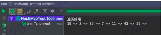
遍历上图的最终结果是 19 -> 3 -> 35 -> 7 -> 11 -> 43 -> 59,为了验证正确性,简单写点测试代码跑一下看看。测试代码如下:
/**
 * 应在 JDK 1.8 下测试,其他环境下不保证结果和上面一致
 */
public class HashMapTest {

    @Test
    public void testTraversal() {
        HashMap<Integer, String> map = new HashMap(16);
        map.put(7, "");
        map.put(11, "");
        map.put(43, "");
        map.put(59, "");
        map.put(19, "");
        map.put(3, "");
        map.put(35, "");

        System.out.println("遍历结果:");
        for (Integer key : map.keySet()) {
            System.out.print(key + " -> ");
        }
    }
}
遍历结果如下:
在本小节的最后,抛两个问题给大家。在 JDK 1.8 版本中,为了避免过长的链表对 HashMap 性能的影响,特地引入了红黑树优化性能。但在上面的源码中并没有发现红黑树遍历的相关逻辑,这是为什么呢?对于被转换成红黑树的链表该如何遍历呢?大家可以先想想,然后可以去源码或本文后续章节中找答案。
11.插入
11.1 插入逻辑分析
通过前两节的分析,大家对HashMap 低层的数据结构应该了然于心了。即使我不说,大家也应该能知道 HashMap 的插入流程是什么样的了。
首先肯定是先定位要插入的键值对属于哪个桶,定位到桶后,再判断桶是否为空。如果为空,则将键值对存入即可。如果不为空,则需将键值对接在链表最后一个位置,或者更新键值对。这就是 HashMap 的插入流程,是不是觉得很简单。
当然,大家先别高兴。这只是一个简化版的插入流程,真正的插入流程要复杂不少。首先 HashMap 是变长集合,所以需要考虑扩容的问题。其次,在 JDK 1.8 中,HashMap 引入了红黑树优化过长链表,这里还要考虑多长的链表需要进行优化,优化过程又是怎样的问题。
引入这里两个问题后,大家会发现原本简单的操作,现在略显复杂了。
在本节中,我将先分析插入操作的源码,扩容、树化(链表转为红黑树,下同)以及其他和树结构相关的操作,随后将在独立的两小结中进行分析。接下来,先来看一下插入操作的源码:
/**
     * Associates the specified value with the specified key in this map.
     * If the map previously contained a mapping for the key, the old
     * value is replaced.
     *
     * @param key key with which the specified value is to be associated
     * @param value value to be associated with the specified key
     * @return the previous value associated with <tt>key</tt>, or
     *         <tt>null</tt> if there was no mapping for <tt>key</tt>.
     *         (A <tt>null</tt> return can also indicate that the map
     *         previously associated <tt>null</tt> with <tt>key</tt>.)
     */
    public V put(K key, V value) {
        return putVal(hash(key), key, value, false, true);
    }


	/**
     * Implements Map.put and related methods.
     *
     * @param hash hash for key
     * @param key the key
     * @param value the value to put
     * @param onlyIfAbsent if true, don't change existing value
     * @param evict if false, the table is in creation mode.
     * @return previous value, or null if none
     */
    final V putVal(int hash, K key, V value, boolean onlyIfAbsent,
                   boolean evict) {
        Node<K,V>[] tab; Node<K,V> p; int n, i;
        // 初始化桶数组 table,table 被延迟到插入新数据时再进行初始化
        if ((tab = table) == null || (n = tab.length) == 0)
            n = (tab = resize()).length;
        // 如果桶中不包含键值对节点引用,则将新键值对节点的引用存入桶中即可
        if ((p = tab[i = (n - 1) & hash]) == null)
            tab[i] = newNode(hash, key, value, null);
        else {
            Node<K,V> e; K k;
             // 如果键的值以及节点 hash 等于链表中的第一个键值对节点时,则将 e 指向该键值对
            if (p.hash == hash &&
                ((k = p.key) == key || (key != null && key.equals(k))))
                e = p;
             // 如果桶中的引用类型为 TreeNode,则调用红黑树的插入方法
            else if (p instanceof TreeNode)
                e = ((TreeNode<K,V>)p).putTreeVal(this, tab, hash, key, value);
            else {
                 // 对链表进行遍历,并统计链表长度
                for (int binCount = 0; ; ++binCount) {
                    // 链表中不包含要插入的键值对节点时,则将该节点接在链表的最后
                    if ((e = p.next) == null) {
                        p.next = newNode(hash, key, value, null);
                        // 如果链表长度大于或等于树化阈值,则进行树化操作
                        if (binCount >= TREEIFY_THRESHOLD - 1) // -1 for 1st
                            treeifyBin(tab, hash);
                        break;
                    }
                     // 条件为 true,表示当前链表包含要插入的键值对,终止遍历
                    if (e.hash == hash &&
                        ((k = e.key) == key || (key != null && key.equals(k))))
                        break;
                    p = e;
                }
            }
            // 判断要插入的键值对是否存在 HashMap 中
            if (e != null) { // existing mapping for key
                V oldValue = e.value;
                 // onlyIfAbsent 表示是否仅在 oldValue 为 null 的情况下更新键值对的值
                if (!onlyIfAbsent || oldValue == null)
                    e.value = value;
                afterNodeAccess(e);
                return oldValue;
            }
        }
        ++modCount;
        // 键值对数量超过阈值时,则进行扩容
        if (++size > threshold)
            resize();
        afterNodeInsertion(evict);
        return null;
    }
插入操作的入口方法是 put(K,V),但核心逻辑在V putVal(int, K, V, boolean, boolean) 方法中。putVal 方法主要做了这么几件事情:
- 当桶数组 table 为空时,通过扩容的方式初始化 table
- 查找要插入的键值对是否已经存在,存在的话根据条件判断是否用新值替换旧值
- 如果不存在,则将键值对链入链表中,并根据链表长度决定是否将链表转为红黑树
- 判断键值对数量是否大于阈值,大于的话则进行扩容操作
以上就是 HashMap 插入的逻辑,并不是很复杂,这里就不多说了。接下来来分析一下扩容机制。
12.扩容机制
在 Java 中,数组的长度是固定的,这意味着数组只能存储固定量的数据。但在开发的过程中,很多时候我们无法知道该建多大的数组合适。建小了不够用,建大了用不完,造成浪费。如果我们能实现一种变长的数组,并按需分配空间就好了。好在,我们不用自己实现变长数组,Java 集合框架已经实现了变长的数据结构。比如 ArrayList 和 HashMap。对于这类基于数组的变长数据结构,扩容是一个非常重要的操作。下面就来聊聊 HashMap 的扩容机制。
在详细分析之前,先来说一下扩容相关的背景知识:
在 HashMap 中,桶数组的长度均是2的幂,阈值大小为桶数组长度与负载因子的乘积。当 HashMap 中的键值对数量超过阈值时,进行扩容。
HashMap 的扩容机制与其他变长集合的套路不太一样,HashMap 按当前桶数组长度的2倍进行扩容,阈值也变为原来的2倍(如果计算过程中,阈值溢出归零,则按阈值公式重新计算)。扩容之后,要重新计算键值对的位置,并把它们移动到合适的位置上去。以上就是 HashMap的扩容大致过程,接下来我们来看看具体的实现:
final Node<K,V>[] resize() {
    Node<K,V>[] oldTab = table;
    int oldCap = (oldTab == null) ? 0 : oldTab.length;
    int oldThr = threshold;
    int newCap, newThr = 0;
    // 如果 table 不为空,表明已经初始化过了
    if (oldCap > 0) {
        // 当 table 容量超过容量最大值,则不再扩容
        if (oldCap >= MAXIMUM_CAPACITY) {
            threshold = Integer.MAX_VALUE;
            return oldTab;
        }
        // 按旧容量和阈值的2倍计算新容量和阈值的大小
        else if ((newCap = oldCap << 1) < MAXIMUM_CAPACITY &&
                 oldCap >= DEFAULT_INITIAL_CAPACITY)
            newThr = oldThr << 1; // double threshold
    } else if (oldThr > 0) // initial capacity was placed in threshold
        /*
         * 初始化时,将 threshold 的值赋值给 newCap,
         * HashMap 使用 threshold 变量暂时保存 initialCapacity 参数的值
         */
        newCap = oldThr;
    else {               // zero initial threshold signifies using defaults
        /*
         * 调用无参构造方法时,桶数组容量为默认容量,
         * 阈值为默认容量与默认负载因子乘积
         */
        newCap = DEFAULT_INITIAL_CAPACITY;
        newThr = (int)(DEFAULT_LOAD_FACTOR * DEFAULT_INITIAL_CAPACITY);
    }

    // newThr 为 0 时,按阈值计算公式进行计算
    if (newThr == 0) {
        float ft = (float)newCap * loadFactor;
        newThr = (newCap < MAXIMUM_CAPACITY && ft < (float)MAXIMUM_CAPACITY ?
                  (int)ft : Integer.MAX_VALUE);
    }
    threshold = newThr;
    // 创建新的桶数组,桶数组的初始化也是在这里完成的
    Node<K,V>[] newTab = (Node<K,V>[])new Node[newCap];
    table = newTab;
    if (oldTab != null) {
        // 如果旧的桶数组不为空,则遍历桶数组,并将键值对映射到新的桶数组中
        for (int j = 0; j < oldCap; ++j) {
            Node<K,V> e;
            if ((e = oldTab[j]) != null) {
                oldTab[j] = null;
                if (e.next == null)
                    newTab[e.hash & (newCap - 1)] = e;
                else if (e instanceof TreeNode)
                    // 重新映射时,需要对红黑树进行拆分
                    ((TreeNode<K,V>)e).split(this, newTab, j, oldCap);
                else { // preserve order
                    Node<K,V> loHead = null, loTail = null;
                    Node<K,V> hiHead = null, hiTail = null;
                    Node<K,V> next;
                    // 遍历链表,并将链表节点按原顺序进行分组
                    do {
                        next = e.next;
                        if ((e.hash & oldCap) == 0) {
                            if (loTail == null)
                                loHead = e;
                            else
                                loTail.next = e;
                            loTail = e;
                        }
                        else {
                            if (hiTail == null)
                                hiHead = e;
                            else
                                hiTail.next = e;
                            hiTail = e;
                        }
                    } while ((e = next) != null);
                    // 将分组后的链表映射到新桶中
                    if (loTail != null) {
                        loTail.next = null;
                        newTab[j] = loHead;
                    }
                    if (hiTail != null) {
                        hiTail.next = null;
                        newTab[j + oldCap] = hiHead;
                    }
                }
            }
        }
    }
    return newTab;
}
上面的源码有点长,希望大家耐心看懂它的逻辑。上面的源码总共做了3件事,分别是:
- 计算新桶数组的容量 newCap 和新阈值 newThr
- 根据计算出的 newCap 创建新的桶数组,桶数组 table 也是在这里进行初始化的
- 将键值对节点重新映射到新的桶数组里。如果节点是 TreeNode 类型,则需要拆分红黑树。如果是普通节点,则节点按原顺序进行分组。
上面列的三点中,创建新的桶数组就一行代码,不用说了。接下来,来说说第一点和第三点,先说说 newCap 和 newThr 计算过程。该计算过程对应 resize 源码的第一和第二个条件分支,如下:
// 第一个条件分支
if ( oldCap > 0) {
    // 嵌套条件分支
    if (oldCap >= MAXIMUM_CAPACITY) {...}
    else if ((newCap = oldCap << 1) < MAXIMUM_CAPACITY &&
                 oldCap >= DEFAULT_INITIAL_CAPACITY) {...}
}
else if (oldThr > 0) {...}
else {...}

// 第二个条件分支
if (newThr == 0) {...}
通过这两个条件分支对不同情况进行判断,进而算出不同的容量值和阈值。它们所覆盖的情况如下:
分支一:
| 条件 | 覆盖情况 | 备注 |
|---|---|---|
| oldCap > 0 | 桶数组 table 已经被初始化 | |
| oldThr > 0 | threshold > 0,且桶数组未被初始化 | 调用 HashMap(int) 和 HashMap(int, float) 构造方法时会产生这种情况,此种情况下 newCap = oldThr,newThr 在第二个条件分支中算出 |
| oldCap == 0 && oldThr == 0 | 桶数组未被初始化,且 threshold 为 0 | 调用 HashMap() 构造方法会产生这种情况。 |
这里把oldThr > 0情况单独拿出来说一下。在这种情况下,会将 oldThr 赋值给 newCap,等价于newCap = threshold = tableSizeFor(initialCapacity)。我们在初始化时传入的 initialCapacity 参数经过 threshold 中转最终赋值给了 newCap。这也就解答了前面提的一个疑问:initialCapacity 参数没有被保存下来,那么它怎么参与桶数组的初始化过程的呢?
嵌套分支:
| 条件 | 覆盖情况 | 备注 |
|---|---|---|
| oldCap >= 230 | 桶数组容量大于或等于最大桶容量 230 | 这种情况下不再扩容 |
| newCap < 230 && oldCap > 16 | 新桶数组容量小于最大值,且旧桶数组容量大于 16 | 该种情况下新阈值 newThr = oldThr << 1,移位可能会导致溢出 |
这里简单说明一下移位导致的溢出情况,当loadFactor小数位为 0,整数位可被2整除且大于等于8时,在某次计算中就可能会导致 newThr溢出归零。见下图

分支二:
| 条件 | 覆盖情况 | 备注 |
|---|---|---|
| newThr == 0 | 第一个条件分支未计算 newThr 或嵌套分支在计算过程中导致 newThr 溢出归零 |
说完 newCap 和 newThr 的计算过程,接下来再来分析一下键值对节点重新映射的过程。
在 JDK 1.8 中,重新映射节点需要考虑节点类型。对于树形节点,需先拆分红黑树再映射。对于链表类型节点,则需先对链表进行分组,然后再映射。需要的注意的是,分组后,组内节点相对位置保持不变。关于红黑树拆分的逻辑将会放在下一小节说明,先来看看链表是怎样进行分组映射的。
我们都知道往底层数据结构中插入节点时,一般都是先通过模运算计算桶位置,接着把节点放入桶中即可。事实上,我们可以把重新映射看做插入操作。在 JDK 1.7 中,也确实是这样做的。但在 JDK 1.8 中,则对这个过程进行了一定的优化,逻辑上要稍微复杂一些。在详细分析前,我们先来回顾一下 hash 求余的过程:

上图中,桶数组大小n = 16,hash1 与 hash2不相等。但因为只有后4位参与求余,所以结果相等。当桶数组扩容后,n 由16变成了32,对上面的 hash 值重新进行映射:
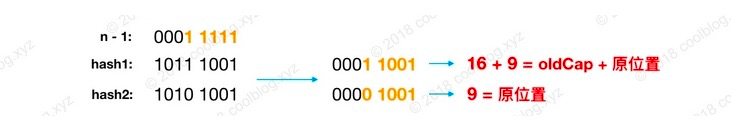
扩容后,参与模运算的位数由4位变为了5位。由于两个 hash 第5位的值是不一样,所以两个hash算出的结果也不一样。上面的计算过程并不难理解,继续往下分析。

假设我们上图的桶数组进行扩容,扩容后容量 n = 16,重新映射过程如下:
依次遍历链表,并计算节点 hash & oldCap 的值。如下图所示

如果值为0,将 loHead 和loTail指向这个节点。如果后面还有节点hash & oldCap 为0的话,则将节点链入loHead 指向的链表中,并将loTail指向该节点。如果值为非0的话,则让 hiHead和hiTail指向该节点。完成遍历后,可能会得到两条链表,此时就完成了链表分组:

最后再将这两条链接存放到相应的桶中,完成扩容。如下图:

从上图可以发现,重新映射后,两条链表中的节点顺序并未发生变化,还是保持了扩容前的顺序。以上就是 JDK 1.8 中 HashMap 扩容的代码讲解。
另外再补充一下,JDK 1.8版本下 HashMap 扩容效率要高于之前版本。如果大家看过JDK 1.7 的源码会发现,JDK 1.7 为了防止因 hash 碰撞引发的拒绝服务攻击,在计算 hash 过程中引入随机种子。以增强 hash 的随机性,使得键值对均匀分布在桶数组中。在扩容过程中,相关方法会根据容量判断是否需要生成新的随机种子,并重新计算所有节点的hash。而在JDK 1.8 中,则通过引入红黑树替代了该种方式。从而避免了多次计算hash 的操作,提高了扩容效率。
本小节的内容讲就先讲到这,接下来,来讲讲链表与红黑树相互转换的过程。
13.链表树化、红黑树链化与拆分
JDK 1.8 对 HashMap 实现进行了改进。最大的改进莫过于在引入了红黑树处理频繁的碰撞,代码复杂度也随之上升。比如,以前只需实现一套针对链表操作的方法即可。而引入红黑树后,需要另外实现红黑树相关的操作。红黑树是一种自平衡的二叉查找树,本身就比较复杂。
在展开说明之前,先把树化的相关代码贴出来,如下:
static final int TREEIFY_THRESHOLD = 8;

/**
 * 当桶数组容量小于该值时,优先进行扩容,而不是树化
 */
static final int MIN_TREEIFY_CAPACITY = 64;

static final class TreeNode<K,V> extends LinkedHashMap.Entry<K,V> {
    TreeNode<K,V> parent;  // red-black tree links
    TreeNode<K,V> left;
    TreeNode<K,V> right;
    TreeNode<K,V> prev;    // needed to unlink next upon deletion
    boolean red;
    TreeNode(int hash, K key, V val, Node<K,V> next) {
        super(hash, key, val, next);
    }
}

/**
 * 将普通节点链表转换成树形节点链表
 */
final void treeifyBin(Node<K,V>[] tab, int hash) {
    int n, index; Node<K,V> e;
    // 桶数组容量小于 MIN_TREEIFY_CAPACITY,优先进行扩容而不是树化
    if (tab == null || (n = tab.length) < MIN_TREEIFY_CAPACITY)
        resize();
    else if ((e = tab[index = (n - 1) & hash]) != null) {
        // hd 为头节点(head),tl 为尾节点(tail)
        TreeNode<K,V> hd = null, tl = null;
        do {
            // 将普通节点替换成树形节点
            TreeNode<K,V> p = replacementTreeNode(e, null);
            if (tl == null)
                hd = p;
            else {
                p.prev = tl;
                tl.next = p;
            }
            tl = p;
        } while ((e = e.next) != null);  // 将普通链表转成由树形节点链表
        if ((tab[index] = hd) != null)
            // 将树形链表转换成红黑树
            hd.treeify(tab);
    }
}

TreeNode<K,V> replacementTreeNode(Node<K,V> p, Node<K,V> next) {
    return new TreeNode<>(p.hash, p.key, p.value, next);
}
在扩容过程中,树化要满足两个条件:
- 链表长度大于等于
TREEIFY_THRESHOLD - 桶数组容量大于等于
MIN_TREEIFY_CAPACITY
第一个条件比较好理解,这里就不说了。这里来说说加入第二个条件的原因,个人觉得原因如下:
当桶数组容量比较小时,键值对节点 hash的碰撞率可能会比较高,进而导致链表长度较长。这个时候应该优先扩容,而不是立马树化。毕竟高碰撞率是因为桶数组容量较小引起的,这个是主因。容量小时,优先扩容可以避免一些列的不必要的树化过程。同时,桶容量较小时,扩容会比较频繁,扩容时需要拆分红黑树并重新映射。所以在桶容量比较小的情况下,将长链表转成红黑树是一件吃力不讨好的事。
回到上面的源码中,我们继续看一下treeifyBin 方法。该方法主要的作用是将普通链表转成为由 TreeNode 型节点组成的链表,并在最后调用 treeify是将该链表转为红黑树。TreeNode 继承自 Node类,所以 TreeNode 仍然包含 next引用,原链表的节点顺序最终通过 next 引用被保存下来。我们假设树化前,链表结构如下:

HashMap 在设计之初,并没有考虑到以后会引入红黑树进行优化。所以并没有像 TreeMap 那样,要求键类实现 comparable 接口或提供相应的比较器。但由于树化过程需要比较两个键对象的大小,在键类没有实现 comparable 接口的情况下,怎么比较键与键之间的大小了就成了一个棘手的问题。为了解决这个问题,HashMap 是做了三步处理,确保可以比较出两个键的大小,如下:
- 比较键与键之间
hash的大小,如果hash相同,继续往下比较 - 检测键类是否实现了
Comparable 接口,如果实现调用compareTo方法进行比较 - 如果仍未比较出大小,就需要进行仲裁了,仲裁方法为
tieBreakOrder(大家自己看源码吧)
ie break 是网球术语,可以理解为加时赛的意思,起这个名字还是挺有意思的。
通过上面三次比较,最终就可以比较出孰大孰小。比较出大小后就可以构造红黑树了,最终构造出的红黑树如下:

橙色的箭头表示TreeNode的 next引用。由于空间有限,prev 引用未画出。可以看出,链表转成红黑树后,原链表的顺序仍然会被引用仍被保留了(红黑树的根节点会被移动到链表的第一位),我们仍然可以按遍历链表的方式去遍历上面的红黑树。这样的结构为后面红黑树的切分以及红黑树转成链表做好了铺垫,我们继续往下分析。
红黑树拆分
扩容后,普通节点需要重新映射,红黑树节点也不例外。按照一般的思路,我们可以先把红黑树转成链表,之后再重新映射链表即可。这种处理方式是大家比较容易想到的,但这样做会损失一定的效率。不同于上面的处理方式,HashMap 实现的思路则是上好佳(上好佳请把广告费打给我)。
如上节所说,在将普通链表转成红黑树时,HashMap 通过两个额外的引用next和 prev保留了原链表的节点顺序。这样再对红黑树进行重新映射时,完全可以按照映射链表的方式进行。这样就避免了将红黑树转成链表后再进行映射,无形中提高了效率。
以上就是红黑树拆分的逻辑,下面看一下具体实现吧:
// 红黑树转链表阈值
static final int UNTREEIFY_THRESHOLD = 6;

final void split(HashMap<K,V> map, Node<K,V>[] tab, int index, int bit) {
    TreeNode<K,V> b = this;
    // Relink into lo and hi lists, preserving order
    TreeNode<K,V> loHead = null, loTail = null;
    TreeNode<K,V> hiHead = null, hiTail = null;
    int lc = 0, hc = 0;
    /*
     * 红黑树节点仍然保留了 next 引用,故仍可以按链表方式遍历红黑树。
     * 下面的循环是对红黑树节点进行分组,与上面类似
     */
    for (TreeNode<K,V> e = b, next; e != null; e = next) {
        next = (TreeNode<K,V>)e.next;
        e.next = null;
        if ((e.hash & bit) == 0) {
            if ((e.prev = loTail) == null)
                loHead = e;
            else
                loTail.next = e;
            loTail = e;
            ++lc;
        }
        else {
            if ((e.prev = hiTail) == null)
                hiHead = e;
            else
                hiTail.next = e;
            hiTail = e;
            ++hc;
        }
    }

    if (loHead != null) {
        // 如果 loHead 不为空,且链表长度小于等于 6,则将红黑树转成链表
        if (lc <= UNTREEIFY_THRESHOLD)
            tab[index] = loHead.untreeify(map);
        else {
            tab[index] = loHead;
            /*
             * hiHead == null 时,表明扩容后,
             * 所有节点仍在原位置,树结构不变,无需重新树化
             */
            if (hiHead != null)
                loHead.treeify(tab);
        }
    }
    // 与上面类似
    if (hiHead != null) {
        if (hc <= UNTREEIFY_THRESHOLD)
            tab[index + bit] = hiHead.untreeify(map);
        else {
            tab[index + bit] = hiHead;
            if (loHead != null)
                hiHead.treeify(tab);
        }
    }
}
从源码上可以看得出,重新映射红黑树的逻辑和重新映射链表的逻辑基本一致。不同的地方在于,重新映射后,会将红黑树拆分成两条由 TreeNode 组成的链表。如果链表长度小于 UNTREEIFY_THRESHOLD,则将链表转换成普通链表。否则根据条件重新将 TreeNode 链表树化。举个例子说明一下,假设扩容后,重新映射上图的红黑树,映射结果如下:

14.红黑树链化
前面说过,红黑树中仍然保留了原链表节点顺序。有了这个前提,再将红黑树转成链表就简单多了,仅需将 TreeNode 链表转成Node 类型的链表即可。相关代码如下:
final Node<K,V> untreeify(HashMap<K,V> map) {
    Node<K,V> hd = null, tl = null;
    // 遍历 TreeNode 链表,并用 Node 替换
    for (Node<K,V> q = this; q != null; q = q.next) {
        // 替换节点类型
        Node<K,V> p = map.replacementNode(q, null);
        if (tl == null)
            hd = p;
        else
            tl.next = p;
        tl = p;
    }
    return hd;
}

Node<K,V> replacementNode(Node<K,V> p, Node<K,V> next) {
    return new Node<>(p.hash, p.key, p.value, next);
}
上面的代码并不复杂,不难理解,这里就不多说了。到此扩容相关内容就说完了,不知道大家理解没。
15.删除
HashMap 的删除操作并不复杂,仅需三个步骤即可完成。第一步是定位桶位置,第二步遍历链表并找到键值相等的节点,第三步删除节点。相关源码如下:
public V remove(Object key) {
    Node<K,V> e;
    return (e = removeNode(hash(key), key, null, false, true)) == null ?
        null : e.value;
}

final Node<K,V> removeNode(int hash, Object key, Object value,
                           boolean matchValue, boolean movable) {
    Node<K,V>[] tab; Node<K,V> p; int n, index;
    if ((tab = table) != null && (n = tab.length) > 0 &&
        // 1. 定位桶位置
        (p = tab[index = (n - 1) & hash]) != null) {
        Node<K,V> node = null, e; K k; V v;
        // 如果键的值与链表第一个节点相等,则将 node 指向该节点
        if (p.hash == hash &&
            ((k = p.key) == key || (key != null && key.equals(k))))
            node = p;
        else if ((e = p.next) != null) {
            // 如果是 TreeNode 类型,调用红黑树的查找逻辑定位待删除节点
            if (p instanceof TreeNode)
                node = ((TreeNode<K,V>)p).getTreeNode(hash, key);
            else {
                // 2. 遍历链表,找到待删除节点
                do {
                    if (e.hash == hash &&
                        ((k = e.key) == key ||
                         (key != null && key.equals(k)))) {
                        node = e;
                        break;
                    }
                    p = e;
                } while ((e = e.next) != null);
            }
        }

        // 3. 删除节点,并修复链表或红黑树
        if (node != null && (!matchValue || (v = node.value) == value ||
                             (value != null && value.equals(v)))) {
            if (node instanceof TreeNode)
                ((TreeNode<K,V>)node).removeTreeNode(this, tab, movable);
            else if (node == p)
                tab[index] = node.next;
            else
                p.next = node.next;
            ++modCount;
            --size;
            afterNodeRemoval(node);
            return node;
        }
    }
    return null;
}
删除操作本身并不复杂,有了前面的基础,理解起来也就不难了,这里就不多说了。
16.其他细节
前面的内容分析了 HashMap 的常用操作及相关的源码,本节内容再补充一点其他方面的东西。
被 transient 所修饰 table 变量
如果大家细心阅读 HashMap 的源码,会发现桶数组 table 被申明为transient。transient 表示易变的意思,在 Java 中,被该关键字修饰的变量不会被默认的序列化机制序列化。
我们再回到源码中,考虑一个问题:桶数组 table 是 HashMap 底层重要的数据结构,不序列化的话,别人还怎么还原呢?
这里简单说明一下吧,HashMap 并没有使用默认的序列化机制,而是通过实现readObject/writeObject两个方法自定义了序列化的内容。这样做是有原因的,试问一句,HashMap 中存储的内容是什么?不用说,大家也知道是键值对。所以只要我们把键值对序列化了,我们就可以根据键值对数据重建 HashMap。有的朋友可能会想,序列化table 不是可以一步到位,后面直接还原不就行了吗?这样一想,倒也是合理。但序列化 talbe存在着两个问题:
- table 多数情况下是无法被存满的,序列化未使用的部分,浪费空间
- 同一个键值对在不同 JVM 下,所处的桶位置可能是不同的,在不同的 JVM 下反序列化 table 可能会发生错误。
以上两个问题中,第一个问题比较好理解,第二个问题解释一下。HashMap 的get/put/remove等方法第一步就是根据 hash 找到键所在的桶位置,但如果键没有覆写 hashCode 方法,计算 hash 时最终调用 Object 中的 hashCode 方法。但 Object 中的 hashCode 方法是 native 型的,不同的 JVM 下,可能会有不同的实现,产生的 hash 可能也是不一样的。也就是说同一个键在不同平台下可能会产生不同的 hash,此时再对在同一个 table 继续操作,就会出现问题。
综上所述,大家应该能明白 HashMap 不序列化 table 的原因了。
17.总结
本章对 HashMap 常见操作相关代码进行了详细分析,并在最后补充了一些其他细节。在本章中,插入操作一节的内容说的最多,主要是因为插入操作涉及的点特别多,一环扣一环。包含但不限于“table 初始化、扩容、树化”等,总体来说,插入操作分析起来难度还是很大的。好在,最后分析完了。
本章篇幅虽比较大,但仍未把 HashMap 所有的点都分析到。比如,红黑树的增删查等操作。当然,我个人看来,以上的分析已经够了。毕竟大家是类库的使用者而不是设计者,没必要去弄懂每个细节。所以如果某些细节实在看不懂的话就跳过吧,对我们开发来说,知道 HashMap 大致原理即可。
好了,本章到此结束。
