作业一
作业内容:
实现k-NN,SVM分类器,Softmax分类器和两层神经网络,实践一个简单的图像分类流程。
多类支持向量机损失 Multiclass Support Vector Machine Loss:


SVM 的损失函数:

如何理解损失函数:
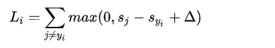
yi 代表正确类别的标签中第i个数据。举个例子来理解SVM的损失函数:假设有3个分类,并且得到了分值[13,-7,11]。其中第一个类别是正确类别,即yi =0;同时假设三角形间隔是10,上面的公式是将所有不正确分类加起来,所以我们得到两个部分:
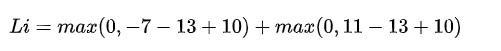
可以看到第一个部分结果是0,这是因为[-7-13+10]得到的是负数,经过max函数处理后得到0。这一对类别分数和标签的损失值是0,这是因为正确分类的得分13与错误分类的得分-7的差为20,高于边界值10。而SVM只关心差距至少要大于10,更大的差值还是算作损失值为0。第二个部分计算[11-13+10]得到8。虽然正确分类的得分比不正确分类的得分要高(13>11),但是比10的边界值还是小了,分差只有2,这就是为什么损失值等于8。简而言之,SVM的损失函数想要正确分类类别[公式]的分数比不正确类别分数高,而且至少要高10。如果不满足这点,就开始计算损失值。
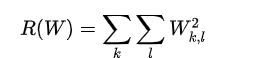
正则化:
我们希望能向某些特定的权重W添加一些偏好,对其他权重则不添加,以此来消除模糊性。这一点是能够实现的,方法是向损失函数增加一个正则化惩罚最常用的正则化惩罚是L2范式,L2范式通过对所有参数进行逐元素的平方惩罚来抑制大数值的权重:
代码
import random
import numpy as np
from cs231n.data_utils import load_CIFAR10
import matplotlib.pyplot as plt

# matplotlib 设置
%matplotlib inline
plt.rcParams['figure.figsize'] = (10.0, 8.0) # set default size of plots
plt.rcParams['image.interpolation'] = 'nearest'
plt.rcParams['image.cmap'] = 'gray'

%load_ext autoreload
%autoreload 2
# 加载 CIFAR-10 数据.
cifar10_dir = 'cs231n/datasets/CIFAR10'

# Cleaning up variables to prevent loading data multiple times (which may cause memory issue)
try:
   del X_train, y_train
   del X_test, y_test
   print('Clear previously loaded data.')
except:
   pass

X_train, y_train, X_test, y_test = load_CIFAR10(cifar10_dir)

# As a sanity check, we print out the size of the training and test data.
print('Training data shape: ', X_train.shape)
print('Training labels shape: ', y_train.shape)
print('Test data shape: ', X_test.shape)
print('Test labels shape: ', y_test.shape)
# 可视化一些训练样本
classes = ['plane', 'car', 'bird', 'cat', 'deer', 'dog', 'frog', 'horse', 'ship', 'truck']
num_classes = len(classes)
samples_per_class = 7
for y, cls in enumerate(classes):
    idxs = np.flatnonzero(y_train == y)
    idxs = np.random.choice(idxs, samples_per_class, replace=False)
    for i, idx in enumerate(idxs):
        plt_idx = i * num_classes + y + 1
        plt.subplot(samples_per_class, num_classes, plt_idx)
        plt.imshow(X_train[idx].astype('uint8'))
        plt.axis('off')
        if i == 0:
            plt.title(cls)
plt.show()
划分训练集、验证集、测试集
# 将数据拆分为训练,验证集和测试集
#创建一个小的开发集作为训练数据的子集
num_training = 49000
num_validation = 1000
num_test = 1000
num_dev = 500

# 验证集.num_training到num_training + num_validation
mask = range(num_training, num_training + num_validation)
X_val = X_train[mask]
y_val = y_train[mask]

#训练集.
mask = range(num_training)
X_train = X_train[mask]
y_train = y_train[mask]

#开发集
mask = np.random.choice(num_training, num_dev, replace=False)
X_dev = X_train[mask]
y_dev = y_train[mask]

#测试集
mask = range(num_test)
X_test = X_test[mask]
y_test = y_test[mask]

print('Train data shape: ', X_train.shape)
print('Train labels shape: ', y_train.shape)
print('Validation data shape: ', X_val.shape)
print('Validation labels shape: ', y_val.shape)
print('Test data shape: ', X_test.shape)
print('Test labels shape: ', y_test.shape)
# 转换shape将图像中的像素变成一行数据 样本*特征
X_train = np.reshape(X_train, (X_train.shape[0], -1))
X_val = np.reshape(X_val, (X_val.shape[0], -1))
X_test = np.reshape(X_test, (X_test.shape[0], -1))
X_dev = np.reshape(X_dev, (X_dev.shape[0], -1))

# 输出
print('Training data shape: ', X_train.shape)
print('Validation data shape: ', X_val.shape)
print('Test data shape: ', X_test.shape)
print('dev data shape: ', X_dev.shape)
预处理阶段
# 预处理:减去平均图像
# 首先:根据训练数据计算图像均值
mean_image = np.mean(X_train, axis=0)
print(mean_image[:10]) # print a few of the elements
plt.figure(figsize=(4,4))
plt.imshow(mean_image.reshape((32,32,3)).astype('uint8')) # visualize the mean image
plt.show()

# 第二:从训练和测试数据中减去平均图像
X_train -= mean_image
X_val -= mean_image
X_test -= mean_image
X_dev -= mean_image


# 第三:附加一个偏置项,以便我们的SVM
# 仅需担心优化单个权重矩阵W
X_train = np.hstack([X_train, np.ones((X_train.shape[0], 1))])
X_val = np.hstack([X_val, np.ones((X_val.shape[0], 1))])
X_test = np.hstack([X_test, np.ones((X_test.shape[0], 1))])
X_dev = np.hstack([X_dev, np.ones((X_dev.shape[0], 1))])

print(X_train.shape, X_val.shape, X_test.shape, X_dev.shape)
分类器:损失函数
from cs231n.classifiers.linear_svm import svm_loss_naive
import time

# 初始化随机权重
W = np.random.randn(3073, 10) * 0.0001

loss, grad = svm_loss_naive(W, X_dev, y_dev, 0.000005)
print('loss: %f' % (loss, ))
# 计算梯度
loss, grad = svm_loss_naive(W, X_dev, y_dev, 0.0)


from cs231n.gradient_check import grad_check_sparse
f = lambda w: svm_loss_naive(w, X_dev, y_dev, 0.0)[0]
grad_numerical = grad_check_sparse(f, W, grad)

# 梯度检测
loss, grad = svm_loss_naive(W, X_dev, y_dev, 5e1)
f = lambda w: svm_loss_naive(w, X_dev, y_dev, 5e1)[0]
grad_numerical = grad_check_sparse(f, W, grad)
比较两种方式:1.向量化 2。矩阵化
# 向量、矩阵形式损失函数,并比较时间
tic = time.time()
loss_naive, grad_naive = svm_loss_naive(W, X_dev, y_dev, 0.000005)
toc = time.time()
print('Naive loss: %e computed in %fs' % (loss_naive, toc - tic))

from cs231n.classifiers.linear_svm import svm_loss_vectorized
tic = time.time()
loss_vectorized, _ = svm_loss_vectorized(W, X_dev, y_dev, 0.000005)
toc = time.time()
print('Vectorized loss: %e computed in %fs' % (loss_vectorized, toc - tic))

print('difference: %f' % (loss_naive - loss_vectorized))
# 向量、矩阵形式梯度,并比较时间
tic = time.time()
_, grad_naive = svm_loss_naive(W, X_dev, y_dev, 0.000005)
toc = time.time()
print('Naive loss and gradient: computed in %fs' % (toc - tic))

tic = time.time()
_, grad_vectorized = svm_loss_vectorized(W, X_dev, y_dev, 0.000005)
toc = time.time()
print('Vectorized loss and gradient: computed in %fs' % (toc - tic))


difference = np.linalg.norm(grad_naive - grad_vectorized, ord='fro')
print('difference: %f' % difference)
训练阶段
from cs231n.classifiers import LinearSVM
svm = LinearSVM()
tic = time.time()
loss_hist = svm.train(X_train, y_train, learning_rate=1e-7, reg=2.5e4,
                      num_iters=1500, verbose=True)
toc = time.time()
print('That took %fs' % (toc - tic))
# 画出图像
plt.plot(loss_hist)
plt.xlabel('Iteration number')
plt.ylabel('Loss value')
plt.show()
预测阶段
# 预测
y_train_pred = svm.predict(X_train)
print('training accuracy: %f' % (np.mean(y_train == y_train_pred), ))
y_val_pred = svm.predict(X_val)
print('validation accuracy: %f' % (np.mean(y_val == y_val_pred), ))
使用验证集调整超参数
# 使用验证集调整超参数(正则化参数和学习率)
learning_rates = [1e-7, 5e-5]
regularization_strengths = [2.5e4, 5e4]


results = {}
best_val = -1
best_svm = None


for learning_rate in learning_rates:
    for regularization_strength in regularization_strengths:
        svm = LinearSVM()
        loss_hist = svm.train(X_train, y_train, learning_rate=learning_rate,
                              reg=regularization_strength, num_iters=1500, verbose=False)
        y_train_pred = svm.predict(X_train)
        training_accuracy = np.mean(y_train == y_train_pred)
        y_val_pred = svm.predict(X_val)
        validation_accuracy = np.mean(y_val == y_val_pred)
        results[(learning_rate, regularization_strength)] = (training_accuracy, validation_accuracy)
        if best_val < validation_accuracy:
            best_val = validation_accuracy
            best_svm = svm

# 打印结果
for lr, reg in sorted(results):
    train_accuracy, val_accuracy = results[(lr, reg)]
    print('lr %e reg %e train accuracy: %f val accuracy: %f' % (
                lr, reg, train_accuracy, val_accuracy))

print('best validation accuracy achieved during cross-validation: %f' % best_val)
# 可视化交叉验证结果
import math
x_scatter = [math.log10(x[0]) for x in results]
y_scatter = [math.log10(x[1]) for x in results]

# 训练集精度
marker_size = 100
colors = [results[x][0] for x in results]
plt.subplot(2, 1, 1)
plt.scatter(x_scatter, y_scatter, marker_size, c=colors, cmap=plt.cm.coolwarm)
plt.colorbar()
plt.xlabel('log learning rate')
plt.ylabel('log regularization strength')
plt.title('CIFAR-10 training accuracy')

# 验证集精度
colors = [results[x][1] for x in results] # default size of markers is 20
plt.subplot(2, 1, 2)
plt.scatter(x_scatter, y_scatter, marker_size, c=colors, cmap=plt.cm.coolwarm)
plt.colorbar()
plt.xlabel('log learning rate')
plt.ylabel('log regularization strength')
plt.title('CIFAR-10 validation accuracy')
plt.show()
测试集
# 测试集
y_test_pred = best_svm.predict(X_test)
test_accuracy = np.mean(y_test == y_test_pred)
print('linear SVM on raw pixels final test set accuracy: %f' % test_accuracy)
可视化每类权重
# 可视化每类权重
w = best_svm.W[:-1,:] # strip out the bias
w = w.reshape(32, 32, 3, 10)
w_min, w_max = np.min(w), np.max(w)
classes = ['plane', 'car', 'bird', 'cat', 'deer', 'dog', 'frog', 'horse', 'ship', 'truck']
for i in range(10):
    plt.subplot(2, 5, i + 1)

    # 把权重映射到0-255
    wimg = 255.0 * (w[:, :, :, i].squeeze() - w_min) / (w_max - w_min)
    plt.imshow(wimg.astype('uint8'))
    plt.axis('off')
    plt.title(classes[i])
linear_classifier.py
from __future__ import print_function

from builtins import range
from builtins import object
import numpy as np
from cs231n.classifiers.linear_svm import *
from cs231n.classifiers.softmax import *
from past.builtins import xrange


class LinearClassifier(object):

    def __init__(self):
        self.W = None

    def train(self, X, y, learning_rate=1e-3, reg=1e-5, num_iters=100,
              batch_size=200, verbose=False):
        """
        Train this linear classifier using stochastic gradient descent.

        Inputs:
        - X: A numpy array of shape (N, D) containing training data; there are N
          training samples each of dimension D.
        - y: A numpy array of shape (N,) containing training labels; y[i] = c
          means that X[i] has label 0 <= c < C for C classes.
        - learning_rate: (float) learning rate for optimization.
        - reg: (float) regularization strength.
        - num_iters: (integer) number of steps to take when optimizing
        - batch_size: (integer) number of training examples to use at each step.
        - verbose: (boolean) If true, print progress during optimization.

        Outputs:
        A list containing the value of the loss function at each training iteration.
        """
        num_train, dim = X.shape
        num_classes = np.max(y) + 1 # assume y takes values 0...K-1 where K is number of classes
        if self.W is None:
            # lazily initialize W
            self.W = 0.001 * np.random.randn(dim, num_classes)

        # Run stochastic gradient descent to optimize W
        loss_history = []
        for it in range(num_iters):
            X_batch = None
            y_batch = None

            #########################################################################
            # TODO:                                                                 #
            # Sample batch_size elements from the training data and their           #
            # corresponding labels to use in this round of gradient descent.        #
            # Store the data in X_batch and their corresponding labels in           #
            # y_batch; after sampling X_batch should have shape (batch_size, dim)   #
            # and y_batch should have shape (batch_size,)                           #
            #                                                                       #
            # Hint: Use np.random.choice to generate indices. Sampling with         #
            # replacement is faster than sampling without replacement.              #
            #########################################################################
            # *****START OF YOUR CODE (DO NOT DELETE/MODIFY THIS LINE)*****

            indices = np.random.choice(num_train,batch_size,replace = False)
            X_batch = X[indices]
            y_batch = y[indices]

            # *****END OF YOUR CODE (DO NOT DELETE/MODIFY THIS LINE)*****

            # evaluate loss and gradient
            loss, grad = self.loss(X_batch, y_batch, reg)
            loss_history.append(loss)

            # perform parameter update
            #########################################################################
            # TODO:                                                                 #
            # Update the weights using the gradient and the learning rate.          #
            #########################################################################
            # *****START OF YOUR CODE (DO NOT DELETE/MODIFY THIS LINE)*****

            loss, grad = self.loss(X_batch, y_batch, reg)
            loss_history.append(loss)
            self.W -= learning_rate*grad

            # *****END OF YOUR CODE (DO NOT DELETE/MODIFY THIS LINE)*****

            if verbose and it % 100 == 0:
                print('iteration %d / %d: loss %f' % (it, num_iters, loss))

        return loss_history

    def predict(self, X):
        """
        Use the trained weights of this linear classifier to predict labels for
        data points.

        Inputs:
        - X: A numpy array of shape (N, D) containing training data; there are N
          training samples each of dimension D.

        Returns:
        - y_pred: Predicted labels for the data in X. y_pred is a 1-dimensional
          array of length N, and each element is an integer giving the predicted
          class.
        """
        y_pred = np.zeros(X.shape[0])
        ###########################################################################
        # TODO:                                                                   #
        # Implement this method. Store the predicted labels in y_pred.            #
        ###########################################################################
        # *****START OF YOUR CODE (DO NOT DELETE/MODIFY THIS LINE)*****

        scores = X.dot(self.W)
        y_pred = np.argsort(scores,axis = 1)[:,-1]

        # *****END OF YOUR CODE (DO NOT DELETE/MODIFY THIS LINE)*****
        return y_pred

    def loss(self, X_batch, y_batch, reg):
        """
        Compute the loss function and its derivative.
        Subclasses will override this.

        Inputs:
        - X_batch: A numpy array of shape (N, D) containing a minibatch of N
          data points; each point has dimension D.
        - y_batch: A numpy array of shape (N,) containing labels for the minibatch.
        - reg: (float) regularization strength.

        Returns: A tuple containing:
        - loss as a single float
        - gradient with respect to self.W; an array of the same shape as W
        """
        pass


class LinearSVM(LinearClassifier):
    """ A subclass that uses the Multiclass SVM loss function """

    def loss(self, X_batch, y_batch, reg):
        return svm_loss_vectorized(self.W, X_batch, y_batch, reg)


class Softmax(LinearClassifier):
    """ A subclass that uses the Softmax + Cross-entropy loss function """

    def loss(self, X_batch, y_batch, reg):
        return softmax_loss_vectorized(self.W, X_batch, y_batch, reg)
linear_svm.py
from builtins import range
import numpy as np
from random import shuffle
from past.builtins import xrange

def svm_loss_naive(W, X, y, reg):
    """
    Structured SVM loss function, naive implementation (with loops).

    Inputs have dimension D, there are C classes, and we operate on minibatches
    of N examples.

    Inputs:
    - W: A numpy array of shape (D, C) containing weights.
    - X: A numpy array of shape (N, D) containing a minibatch of data.
    - y: A numpy array of shape (N,) containing training labels; y[i] = c means
      that X[i] has label c, where 0 <= c < C.
    - reg: (float) regularization strength

    Returns a tuple of:
    - loss as single float
    - gradient with respect to weights W; an array of same shape as W
    """
    dW = np.zeros(W.shape) # initialize the gradient as zero

    # compute the loss and the gradient
    num_classes = W.shape[1]
    num_train = X.shape[0]
    loss = 0.0
    for i in range(num_train):
        scores = X[i].dot(W)
        correct_class_score = scores[y[i]]
        for j in range(num_classes):
            if j == y[i]:
                continue
            margin = scores[j] - correct_class_score + 1 # note delta = 1
            if margin > 0:
                loss += margin

    # Right now the loss is a sum over all training examples, but we want it
    # to be an average instead so we divide by num_train.
    loss /= num_train

    # Add regularization to the loss.
    loss += reg * np.sum(W * W)

    #############################################################################
    # TODO:                                                                     #
    # Compute the gradient of the loss function and store it dW.                #
    # Rather that first computing the loss and then computing the derivative,   #
    # it may be simpler to compute the derivative at the same time that the     #
    # loss is being computed. As a result you may need to modify some of the    #
    # code above to compute the gradient.                                       #
    #############################################################################
    # *****START OF YOUR CODE (DO NOT DELETE/MODIFY THIS LINE)*****

    for i in range(num_train):
        scores = X[i].dot(W)
        index = y[i]
        for j in range(num_classes):
            if j != index and scores[j] >= scores[index]-1:
                dW[:,j] += X[i]
                dW[:,index] -= X[i]

    dW /= num_train
    dW += 2*reg*W

    # *****END OF YOUR CODE (DO NOT DELETE/MODIFY THIS LINE)*****

    return loss, dW


def svm_loss_vectorized(W, X, y, reg):
    """
    Structured SVM loss function, vectorized implementation.

    Inputs and outputs are the same as svm_loss_naive.
    """
    loss = 0.0
    dW = np.zeros(W.shape) # initialize the gradient as zero

    #############################################################################
    # TODO:                                                                     #
    # Implement a vectorized version of the structured SVM loss, storing the    #
    # result in loss.                                                           #
    #############################################################################
    # *****START OF YOUR CODE (DO NOT DELETE/MODIFY THIS LINE)*****

    num_train = X.shape[0]
    scores = X.dot(W)
    rightscore = scores[np.arange(num_train), y]
    scores = scores - rightscore.reshape(-1, 1) + 1.
    scores[scores <= 0] = 0
    scores[np.arange(num_train), y] = 0
    loss = np.sum(scores)/num_train

    # *****END OF YOUR CODE (DO NOT DELETE/MODIFY THIS LINE)*****

    #############################################################################
    # TODO:                                                                     #
    # Implement a vectorized version of the gradient for the structured SVM     #
    # loss, storing the result in dW.                                           #
    #                                                                           #
    # Hint: Instead of computing the gradient from scratch, it may be easier    #
    # to reuse some of the intermediate values that you used to compute the     #
    # loss.                                                                     #
    #############################################################################
    # *****START OF YOUR CODE (DO NOT DELETE/MODIFY THIS LINE)*****

    C = W.shape[1]
    mask = np.zeros((num_train, C))
    scores[scores > 0] = 1
    mask += scores
    mask[np.arange(num_train), y] = -np.sum(scores,axis = 1)
    dW = X.T.dot(mask)/num_train
    dW += 2*reg*W

    # *****END OF YOUR CODE (DO NOT DELETE/MODIFY THIS LINE)*****

    return loss, dW
参考资料
1.https://blog.csdn.net/Zhuanzhu22nian/article/details/92018949
2.周志华机器学习
3.https://zhuanlan.zhihu.com/p/21930884