前言
本节学习逻辑回归
- 解决分类问题
- 样本特征和发生概率联系在一起
最后涉及多分类的OvR和OvO
1、逻辑回归
将样本的特征和样本发生的概率联系在一起

用到了sigmoid函数

通过训练得到θ
然后可以进行预测
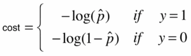
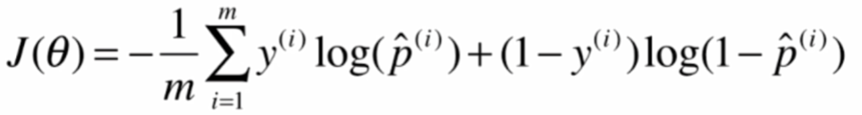
损失函数是
进行演化和代入如下

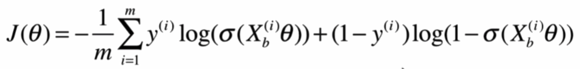
由于这个损失函数没有解析解
所以用梯度下降法来求解
梯度是

实现如下
import numpy as np
from sklearn.metrics import accuracy_score

class LogisticRegression:
    def __init__(self):
        """初始化Logistic Regression模型"""
        self.coef_ = None
        self.intercept_ = None
        self._theta = None

    def _sigmoid(self, t):
        return 1. / (1. + np.exp(-t))

    def fit(self, X_train, y_train, eta=0.01, n_iters=1e4):
        """根据训练数据集X_train, y_train, 使用梯度下降法训练Logistic Regression模型"""
        assert X_train.shape[0] == y_train.shape[0], \
            "the size of X_train must be equal to the size of y_train"
        # 损失函数
        def J(theta, X_b, y):
            y_hat = self._sigmoid(X_b.dot(theta))
            try:
                return - np.sum(y*np.log(y_hat) + (1-y)*np.log(1-y_hat)) / len(y)
            except:
                return float('inf')
        # 梯度
        def dJ(theta, X_b, y):
            return X_b.T.dot(self._sigmoid(X_b.dot(theta)) - y) / len(y)
        # 梯度下降
        def gradient_descent(X_b, y, initial_theta, eta, n_iters=1e4, epsilon=1e-8):
            theta = initial_theta
            cur_iter = 0
            while cur_iter < n_iters:
                gradient = dJ(theta, X_b, y)
                last_theta = theta
                theta = theta - eta * gradient
                if (abs(J(theta, X_b, y) - J(last_theta, X_b, y)) < epsilon):
                    break
                cur_iter += 1
            return theta
        X_b = np.hstack([np.ones((len(X_train), 1)), X_train])
        initial_theta = np.zeros(X_b.shape[1])
        self._theta = gradient_descent(X_b, y_train, initial_theta, eta, n_iters)
        self.intercept_ = self._theta[0]
        self.coef_ = self._theta[1:]
        return self

    def predict_proba(self, X_predict):
        """给定待预测数据集X_predict,返回表示X_predict的结果概率向量"""
        assert self.intercept_ is not None and self.coef_ is not None, \
            "must fit before predict!"
        assert X_predict.shape[1] == len(self.coef_), \
            "the feature number of X_predict must be equal to X_train"
        X_b = np.hstack([np.ones((len(X_predict), 1)), X_predict])
        return self._sigmoid(X_b.dot(self._theta))

    def predict(self, X_predict):
        """给定待预测数据集X_predict,返回表示X_predict的结果向量"""
        assert self.intercept_ is not None and self.coef_ is not None, \
            "must fit before predict!"
        assert X_predict.shape[1] == len(self.coef_), \
            "the feature number of X_predict must be equal to X_train"
        proba = self.predict_proba(X_predict)
        return np.array(proba >= 0.5, dtype='int') #布尔向量

    def score(self, X_test, y_test):
        """根据测试数据集 X_test 和 y_test 确定当前模型的准确度"""
        y_predict = self.predict(X_test)
        return accuracy_score(y_test, y_predict)

    def __repr__(self):
        return "LogisticRegression()"
2、决策边界
通过scikit库来实现逻辑回归
并将决策边界可视化
import numpy as np
import matplotlib.pyplot as plt
from sklearn.model_selection import train_test_split
from sklearn.linear_model import LogisticRegression
from sklearn.preprocessing import PolynomialFeatures
from sklearn.pipeline import Pipeline
from sklearn.preprocessing import StandardScaler

"""用scikit库实现逻辑回归"""
# 数据
np.random.seed(666)
X = np.random.normal(0, 1, size=(200, 2))
y = np.array((X[:, 0] ** 2 + X[:, 1]) < 1.5, dtype='int')
for _ in range(20):
    y[np.random.randint(200)] = 1 #噪音
plt.scatter(X[y == 0, 0], X[y == 0, 1])
plt.scatter(X[y == 1, 0], X[y == 1, 1])
plt.show()
X_train, X_test, y_train, y_test = train_test_split(X, y, random_state=666)
# 逻辑回归
log_reg = LogisticRegression()
log_reg.fit(X_train, y_train)
print(log_reg.score(X_train, y_train))
print(log_reg.score(X_test, y_test))

# 决策边界可视化
def plot_decision_boundary(model, axis):
    x0, x1 = np.meshgrid(
        np.linspace(axis[0], axis[1], int((axis[1] - axis[0]) * 100)).reshape(-1, 1),
        np.linspace(axis[2], axis[3], int((axis[3] - axis[2]) * 100)).reshape(-1, 1),
    )
    X_new = np.c_[x0.ravel(), x1.ravel()]
    y_predict = model.predict(X_new)
    zz = y_predict.reshape(x0.shape)
    from matplotlib.colors import ListedColormap
    custom_cmap = ListedColormap(['#EF9A9A', '#FFF59D', '#90CAF9'])
    plt.contourf(x0, x1, zz, linewidth=5, cmap=custom_cmap)
plot_decision_boundary(log_reg, axis=[-4, 4, -4, 4])
plt.scatter(X[y == 0, 0], X[y == 0, 1])
plt.scatter(X[y == 1, 0], X[y == 1, 1])
plt.show()

# 添加多项式特征
def PolynomialLogisticRegression(degree):
    return Pipeline([
        ('poly', PolynomialFeatures(degree=degree)),
        ('std_scaler', StandardScaler()),
        ('log_reg', LogisticRegression())
    ])
poly_log_reg = PolynomialLogisticRegression(degree=2)
poly_log_reg.fit(X_train, y_train)
print(poly_log_reg.score(X_train, y_train))
print(poly_log_reg.score(X_test, y_test))
plot_decision_boundary(poly_log_reg, axis=[-4, 4, -4, 4])
plt.scatter(X[y == 0, 0], X[y == 0, 1])
plt.scatter(X[y == 1, 0], X[y == 1, 1])
plt.show()
# 20个特征
poly_log_reg2 = PolynomialLogisticRegression(degree=20)
poly_log_reg2.fit(X_train, y_train)
print(poly_log_reg2.score(X_train, y_train))
print(poly_log_reg2.score(X_test, y_test))
plot_decision_boundary(poly_log_reg2, axis=[-4, 4, -4, 4])
plt.scatter(X[y == 0, 0], X[y == 0, 1])
plt.scatter(X[y == 1, 0], X[y == 1, 1])
plt.show()

# 调整分类准确度
def PolynomialLogisticRegression(degree, C):
    return Pipeline([
        ('poly', PolynomialFeatures(degree=degree)),
        ('std_scaler', StandardScaler()),
        ('log_reg', LogisticRegression(C=C))
    ])
poly_log_reg3 = PolynomialLogisticRegression(degree=20, C=0.1)
poly_log_reg3.fit(X_train, y_train)
print(poly_log_reg3.score(X_train, y_train))
print(poly_log_reg3.score(X_test, y_test))
plot_decision_boundary(poly_log_reg3, axis=[-4, 4, -4, 4])
plt.scatter(X[y == 0, 0], X[y == 0, 1])
plt.scatter(X[y == 1, 0], X[y == 1, 1])
plt.show()
得到的几个图依次是
数据

逻辑回归

添加2个多项式特征

添加20个多项式特征

调整分类准确度

3、多分类
多分类有两种办法
- OvO:两两捉对比较特征,资源消耗大,准确
- OvR:提取一种特征,将其他所有座位第二种特征,资源消耗小,但准确性有问题
import numpy as np
import matplotlib.pyplot as plt
from sklearn import datasets
from sklearn.model_selection import train_test_split
from sklearn.linear_model import LogisticRegression

""" 多分类 OvO和OvR"""
# 数据
iris = datasets.load_iris()
X = iris.data[:,:2]
y = iris.target
X_train, X_test, y_train, y_test = train_test_split(X, y, random_state=666)
# 决策边界
def plot_decision_boundary(model, axis):
    x0, x1 = np.meshgrid(
        np.linspace(axis[0], axis[1], int((axis[1] - axis[0]) * 100)).reshape(-1, 1),
        np.linspace(axis[2], axis[3], int((axis[3] - axis[2]) * 100)).reshape(-1, 1),
    )
    X_new = np.c_[x0.ravel(), x1.ravel()]
    y_predict = model.predict(X_new)
    zz = y_predict.reshape(x0.shape)
    from matplotlib.colors import ListedColormap
    custom_cmap = ListedColormap(['#EF9A9A', '#FFF59D', '#90CAF9'])
    plt.contourf(x0, x1, zz, linewidth=5, cmap=custom_cmap)

# OvR
log_reg = LogisticRegression()
log_reg.fit(X_train, y_train)
print(log_reg.score(X_test, y_test))
plot_decision_boundary(log_reg, axis=[4, 8.5, 1.5, 4.5])
plt.scatter(X[y==0,0], X[y==0,1])
plt.scatter(X[y==1,0], X[y==1,1])
plt.scatter(X[y==2,0], X[y==2,1])
plt.show()

# OvO
log_reg2 = LogisticRegression(multi_class="multinomial", solver="newton-cg")
log_reg2.fit(X_train, y_train)
print(log_reg2.score(X_test, y_test))
plot_decision_boundary(log_reg2, axis=[4, 8.5, 1.5, 4.5])
plt.scatter(X[y==0,0], X[y==0,1])
plt.scatter(X[y==1,0], X[y==1,1])
plt.scatter(X[y==2,0], X[y==2,1])
plt.show()
得到的结果如下
OvR

OvO

结语
逻辑回归应该算是机器学习里用的很多的一种算法
对多分类问题做了一定了解